
◆ Research Methods
How do you read multiple regression coefficients, R² and assumptions?
Multiple linear regression predicts one continuous outcome from two or more predictors, and a dissertation chapter usually reports three things from it: how well the whole model fits, what each coefficient says once the other predictors are held constant, and whether the assumptions behind those numbers hold. Most marking comments on regression chapters land on the second and third points rather than on the first.
This guide walks through the equation, the three SPSS tables you will actually report, a worked example of multicollinearity from a published paper, and a checklist of assumptions. It is written for UK and Australian students running their first model, and it pairs with our guide to effect sizes and confidence intervals for the reporting stage.
◆ Question 1 / 7 · The formula
What is the multiple linear regression formula?
Direct answer: The model is Y = b0 + b1X1 + b2X2 + ... + bkXk + e, where b0 is the intercept, each b is the change in Y for a one-unit rise in that predictor with the others held constant, and e is the residual error the predictors leave unexplained (Field, 2024; Bevans, 2023).
Each coefficient therefore answers a conditional question. In a model predicting exam marks from revision hours and lecture attendance, the revision coefficient tells you how much marks change per extra hour among students with the same attendance, which is a different quantity from the simple correlation between revision and marks. That conditional reading is the main reason supervisors ask for multiple rather than simple regression: it separates the contribution of one predictor from the contribution of predictors that travel with it.
The intercept is the predicted outcome when every predictor equals zero. In many student datasets zero is outside the observed range (nobody scored zero on a 1 to 7 Likert scale), so the intercept is needed for the equation but rarely worth interpreting in your discussion. Kim (2019) shows a real fitted equation of this shape for a liver regeneration study, with an intercept of 232.797 and six predictor coefficients.
◆ Question 2 / 7 · Simple vs multiple
How is multiple regression different from simple linear regression?
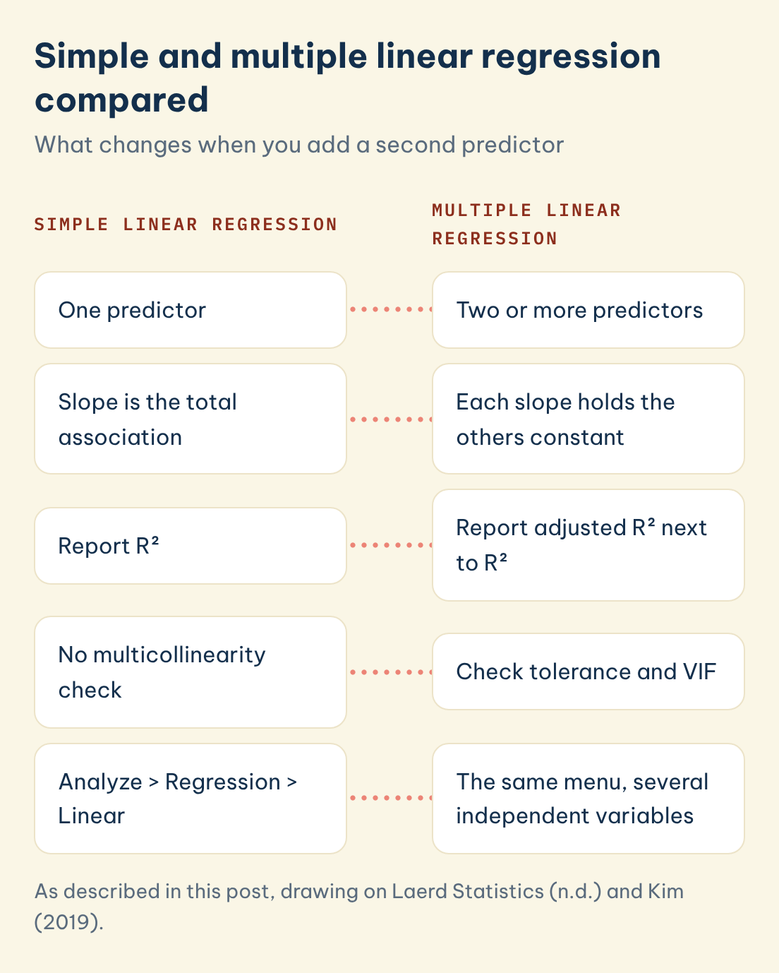
Direct answer: Simple linear regression uses one predictor, so its slope mixes that predictor's effect with everything correlated with it. Multiple regression adds further predictors, so each slope becomes a partial effect, and the model needs extra checks, chiefly multicollinearity, that a one-predictor model cannot have (Laerd Statistics, n.d.; Kim, 2019).
| Feature | Simple linear regression | Multiple linear regression |
|---|---|---|
| Predictors | One | Two or more |
| Meaning of a slope | Total association with the outcome | Association with the others held constant |
| Fit statistic to report | R² | Adjusted R², alongside R² |
| Multicollinearity check | Not applicable | Required (VIF, tolerance) |
| Typical SPSS menu | Analyze > Regression > Linear | The same menu, with several independent variables |
Simple and multiple linear regression compared
What changes when you add a second predictor
Simple linear regression
Multiple linear regression
One predictor
Two or more predictors
Slope is the total association
Each slope holds the others constant
Report R²
Report adjusted R² next to R²
No multicollinearity check
Check tolerance and VIF
Analyze > Regression > Linear
The same menu, several independent variables
Save this figure
The partial meaning can flip a sign. Kim (2019) reports a predictor that was positively related to the outcome in simple regression but carried a negative, non-significant coefficient of -0.050 once five other correlated predictors entered the model. A sign change of this kind is not a software error. The coefficient is answering a narrower question, and when predictors overlap heavily the answer becomes unstable, which is the multicollinearity problem covered below. If you are still deciding whether regression is the right analysis at all, start with our guide to choosing the right statistical test. If your outcome is a yes or no category instead of a score, the same logic carries over to binary logistic regression and odds ratios.
◆ Question 3 / 7 · Reading SPSS output
How do you read multiple linear regression output in SPSS?
Direct answer: Read three tables in order. Model Summary gives R, R² and adjusted R² for overall fit. ANOVA gives the F test of whether the predictors together explain any variance. Coefficients gives each unstandardised B, its standard error, standardised beta, t and p value (Laerd Statistics, n.d.).
Laerd Statistics (n.d.) uses a worked example predicting VO2 max, where R is 0.760 and R² is 0.577, meaning the predictors explain 57.7% of the variability in the outcome. R is the multiple correlation between observed scores and the scores the model predicts. R² is that value squared and is read as a proportion of variance explained. Adjusted R² shrinks R² to correct for the number of predictors, because sample R² tends to overestimate the population value, so it is worth reporting next to R² whenever the model has several predictors.
| SPSS column | What it tells you | How to write it up |
|---|---|---|
| R² | Share of outcome variance the model explains | "explained 57.7% of the variance" |
| Adjusted R² | R² corrected for the number of predictors | Report next to R² |
| F and its p value | Whether the model beats an intercept-only model | F(df1, df2) = value, p = value |
| B (unstandardised) | Change in outcome per unit of the predictor | Interpret in the original units |
| Beta (standardised) | Change in standard deviations, comparable across predictors | Use to compare predictor strength |
| t and p | Whether that single coefficient differs from zero | Report with B and its confidence interval |
Use B when the units mean something to a reader (marks per hour of revision) and beta when you want to compare predictors measured on different scales. Report a confidence interval for each B, because the interval shows how precisely the effect was estimated in a way a lone p value cannot.
◆ Question 4 / 7 · Assumptions
What are the assumptions of multiple linear regression?
Direct answer: Laerd Statistics (n.d.) lists eight: a continuous outcome, two or more predictors, independent residuals, linear relationships, homoscedasticity, no multicollinearity, no influential outliers, and approximately normal residuals. The last four are checked after the model is fitted, using residual plots, VIF values and Cook's distance.
| Assumption | How to check it in SPSS | What a problem looks like |
|---|---|---|
| Independence of residuals | Durbin-Watson statistic | Values far from 2, meaningful only when the data have an order such as time |
| Linearity | Scatterplots and partial regression plots | A curved pattern |
| Homoscedasticity | Studentised residuals against predicted values | A funnel shape |
| No multicollinearity | Tolerance and VIF in the Coefficients table | VIF above 5 to 10 |
| No influential cases | Casewise diagnostics, Cook's distance | A few cases moving the line |
| Normal residuals | Histogram, P-P or Q-Q plot of residuals | Heavy skew or long tails |
One misunderstanding costs students marks repeatedly. The normality assumption concerns the residuals, not the raw predictors or the raw outcome. Ernst and Albers (2017) reviewed regression practice in clinical psychology journals and found that 92% of papers were unclear about how they checked the assumptions, and that some papers wrongly treated normality of the variables, instead of the errors, as the assumption. If your methods chapter says you tested each variable for normality before running regression, a marker may read that as a misunderstanding of the model, so state that you inspected the residual plots instead.
The sample size you need is a separate question from the assumptions. Green (1991) proposed a minimum of 50 + 8m cases for testing the overall model, where m is the number of predictors, so a model with 5 predictors needs at least 90 cases by that rule. Treat it as a floor and check it against a power analysis for your expected effect size.
◆ Question 5 / 7 · Multicollinearity example
What does a multiple regression example with multicollinearity look like?
Direct answer: Kim (2019) fitted six predictors of liver regeneration and found variance inflation factors of 7.387, 6.011 and 4.948 for three of them. After two overlapping predictors were removed, every VIF fell below 2 and a previously non-significant coefficient became significant, while R² barely moved from 0.682 to 0.669.
Kim defines the problem in the article's abstract: "Multicollinearity is present when the VIF is higher than 5 to 10 or the condition indices are higher than 10 to 30" (Kim, 2019, p. 558). The variance inflation factor equals 1 divided by (1 minus R²), where that R² comes from predicting one predictor from all the others. In Kim's six-predictor model the graft-to-standard liver volume ratio had a VIF of 7.387, the graft-to-recipient weight ratio 6.011 and peak systolic velocity 4.948, all at or close to that range. A high VIF inflates the standard error of the coefficient, widens its confidence interval and shrinks its t value, so a real effect can look non-significant.
| Graft-to-recipient weight ratio | Six-predictor model | Four-predictor model |
|---|---|---|
| Variance inflation factor | 6.011 | 1.137 |
| Standard error | 32.665 | 14.014 |
| 95% confidence interval | -104.400 to 29.213 | -97.413 to -40.251 |
| p value | 0.259 | < 0.001 |
| Model R² | 0.682 | 0.669 |
The lesson for a dissertation is in the last row. Dropping the redundant predictors cost almost nothing in explained variance yet turned an uninterpretable coefficient into a precise one. Kim (2019) also warns that removing variables your theory says matter produces biased coefficients, a problem more serious than multicollinearity, so justify any removal on conceptual grounds as well as on the VIF. The diagnostic itself is explained in multicollinearity and the variance inflation factor.
◆ Question 6 / 7 · Python and Excel
Can you run multiple linear regression in Python or Excel?
Direct answer: Yes. Python's statsmodels library fits ordinary least squares models with a summary table of coefficients, R² and diagnostics, and Excel's Analysis ToolPak runs a regression from the Data tab. SPSS is convenient because it produces the assumption checks in the same run.
Whichever software you use, the numbers you report are the same: adjusted R², the F test, and B with its standard error, confidence interval and p value for each predictor. What changes is how much of the assumption checking you must do by hand. Excel's ToolPak, once switched on under File > Options > Add-ins, gives coefficients and residuals but no VIF, so you would compute tolerance separately, while statsmodels provides a variance inflation factor function in its outliers and influence module (statsmodels developers, n.d.). Name the software and version in your methods section, because examiners and journal reviewers expect the analysis to be reproducible from that description.
If your course requires SPSS output, run the final model there even if you explored the data in Python first, so that the tables in your appendix match the figures in your text.
◆ Question 7 / 7 · Mentor help
Can a mentor help you check your regression chapter?
Most students can run the model; the harder part is defending the choices around it. In SPSS, R and Python help for your discipline, a MAAS expert reviews your model specification, assumption checks and write-up with you, and explains each table so you can answer questions on it in a viva or a supervision meeting. You stay responsible for the analysis and the interpretation. Bring your research questions, your variable list and the output you already have to the first session.
Frequently asked questions
What is a good R² in multiple regression?
No single threshold applies, because acceptable values differ by field. Laerd Statistics (n.d.) describes the R of 0.760 in its worked example as a good level of prediction, but in much social science research far smaller values are normal, so compare against published studies in your area.
Should I report R² or adjusted R²?
Report both, and interpret adjusted R² when you have several predictors, because it corrects for the tendency of R² to rise whenever a predictor is added (Field, 2024).
What VIF value indicates multicollinearity?
Kim (2019) treats a VIF above 5 to 10, or a tolerance below 0.1 to 0.2, as a sign of multicollinearity. State the threshold you used and cite its source.
Do my predictors need to be normally distributed?
No. The assumption applies to the residuals of the model, which you check with a histogram or Q-Q plot after fitting it (Ernst & Albers, 2017).
How many participants do I need for multiple regression?
Green (1991) suggests at least 50 + 8m, where m is the number of predictors, as a minimum for testing the overall model. A power analysis based on your expected effect size gives a better answer.
What is the difference between B and beta in SPSS?
B is the unstandardised coefficient in the original units of the variables. Beta is standardised, so it lets you compare predictors measured on different scales (Laerd Statistics, n.d.).
References
Bevans, R. (2023, June 22). Multiple linear regression: A quick guide (examples). Scribbr. https://www.scribbr.com/statistics/multiple-linear-regression/
Ernst, A. F., & Albers, C. J. (2017). Regression assumptions in clinical psychology research practice: A systematic review of common misconceptions. PeerJ, 5, e3323. https://doi.org/10.7717/peerj.3323
Field, A. (2024). Discovering statistics using IBM SPSS Statistics (6th ed.). SAGE.
Green, S. B. (1991). How many subjects does it take to do a regression analysis? Multivariate Behavioral Research, 26(3), 499–510. https://doi.org/10.1207/s15327906mbr2603_7
Kim, J. H. (2019). Multicollinearity and misleading statistical results. Korean Journal of Anesthesiology, 72(6), 558–569. https://doi.org/10.4097/kja.19087
Laerd Statistics. (n.d.). Multiple regression analysis using SPSS Statistics. https://statistics.laerd.com/spss-tutorials/multiple-regression-using-spss-statistics.php
statsmodels developers. (n.d.). Regression diagnostics. statsmodels documentation. https://www.statsmodels.org/stable/diagnostic.html
Tools & resources
Not sure how this guide applies to your own case? Talk it through with MAAS in a free 20-minute consultation.
Book a free consultation ▸