How do you calculate the sample size for a research study?

Calculating the sample size for a research study means working out how many participants you need to detect a real effect before collecting data. You fix your target power, significance level, and expected effect size, and the required number follows.

Get it wrong and the consequences are expensive: too few participants and a true effect stays invisible, wasting months of work; too many and you spend resources you did not need and raise ethical questions about over-recruiting. For Vietnamese researchers aiming at a Scopus Q1 or Q2 journal, a clear sample-size justification is one of the first things a methodological reviewer checks. This guide answers the seven questions Vietnamese researchers ask MAAS publishing mentors most often when they reach the design stage.

Author: MAAS Research Methods Publishing Desk · Reviewed by a Principal Publishing Advisor (PhD in Epidemiology and Biostatistics, Scopus Q1 author and reviewer)
Last updated: 2026-06-10
Category: research-methods

What is a sample size and why does it decide whether you get published?

Direct answer: Your sample size is the number of observations — patients, students, survey respondents — you collect. It matters because statistical power depends on it: an underpowered study can miss a real effect entirely, producing a false negative. Reviewers treat sample-size justification as a marker of a serious, reproducible design, so the calculation belongs in your protocol, not your discussion.

Evidence: Hickey et al. (2018) describe the sample-size calculation as a core part of trial design and warn that small studies "may possess insufficient power to detect a clinically significant difference, if such a difference exists." Serdar et al. (2021) add that an undersized study risks a Type II error while a needlessly large one wastes resources and raises ethical concerns — both are design failures a reviewer can see.

Example: A MAAS Publishing Advisory client planned a two-group quasi-experiment with 24 participants per arm because that was who she could recruit. A 20-minute design review showed her target effect needed roughly 64 per arm for 80% power. She redesigned the recruitment window before collecting a single data point — far cheaper than discovering the problem at peer review.

What three numbers do you need before you can calculate a sample size?

Direct answer: An a priori (before-data) calculation needs three inputs, and the software solves for the fourth — the sample size. You set the significance level (alpha, usually 0.05), the statistical power (usually 0.80, meaning an 80% chance of detecting a true effect), and the expected effect size. Fix any three and the required N follows.

Evidence: Kang (2021) sets out the same four interlinked quantities — alpha, power, effect size, and sample size — and notes that fixing three determines the fourth, with 0.05 and 0.80 as the conventional defaults in health-professions research. Cohen (1992) is the original source of the widely used 0.80 power convention, framed as accepting a Type II error rate four times the Type I rate.

Example: A first-time Vietnamese author told a MAAS mentor he "just wanted a big enough sample." The mentor reframed it as three decisions: how sure do you want to be you are not crying wolf (alpha), how sure that you will catch a real effect (power), and how large an effect is worth catching. With those three set at 0.05, 0.80, and a medium effect, his required N fell out in two minutes.

How do you choose an effect size when you have no pilot data?

Direct answer: The effect size is the hardest input and the one that most changes your N — the smaller the effect you want to detect, the more participants you need. Estimate it three ways, in order of preference: from a similar published study, from a small pilot, or — as a last resort — from Cohen's conventional small/medium/large benchmarks. Always justify your choice in writing.

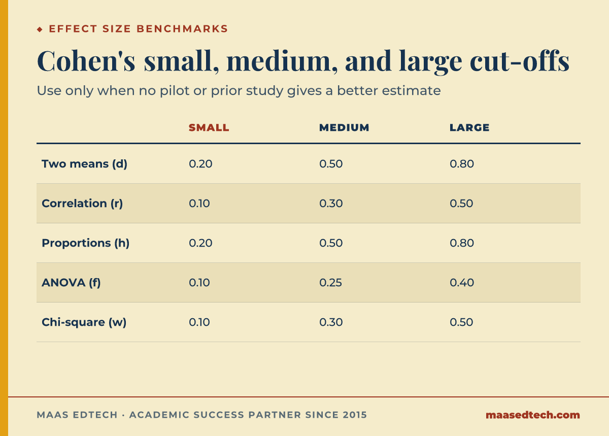
Evidence: Serdar et al. (2021) recommend deriving the expected effect from prior literature or a pilot wherever possible, using standardised benchmarks only when no better estimate exists. Cohen (1992) provides the conventional cut-offs that researchers fall back on, summarised below.

Example: A MAAS-coached health-sciences student had no pilot and no closely matched study. Rather than default to a flattering "large" effect (which would have justified a tiny, underpowered sample of about 26), her mentor helped her locate two comparable papers reporting a Cohen's d near 0.45. Powering for that more honest effect set her target at 158 participants — defensible to any reviewer.

How do you actually run the calculation in G*Power?

Direct answer: G*Power is free, widely accepted, and handles most common designs. The workflow is: choose the statistical test that matches your analysis, set the test family, enter alpha, power, and effect size, then click Calculate to get the required N. The single most common mistake is selecting a test that does not match the analysis you will actually run.

Evidence: Kang (2021) and Faul et al. (2007) — the team behind the software — both stress that the chosen test in G*Power must mirror the planned analysis (t-test, ANOVA, regression, chi-square), because each test has its own power function and effect-size metric. Picking the wrong family silently produces the wrong number.

Example: A Vietnamese master's student ran her power analysis as an independent-samples t-test but planned to analyse her data with a repeated-measures ANOVA. A MAAS mentor caught the mismatch during an Outline → Draft → Final review; correcting the test family in G*Power changed her required sample by nearly 30%. She fixed it before recruitment rather than in a revision letter.

How do you adjust the number for dropout and non-response?

Direct answer: The N from G*Power is the number you need to analyse, not the number to recruit. Inflate it for expected attrition: divide your target by (1 minus the dropout proportion). If you need 100 completers and expect 20% dropout, recruit 100 ÷ 0.80 = 125. Survey studies do the same for the expected non-response rate.

Evidence: Hickey et al. (2018) note that real studies lose participants to withdrawal, loss to follow-up, and missing data, so the recruited sample must exceed the calculated analytic sample. Serdar et al. (2021) similarly advise building an attrition allowance into the recruitment target rather than discovering the shortfall mid-study.

Example: A MAAS Publishing Advisory client running a 12-week intervention calculated 88 completers for 80% power. Vietnamese cohort data from a colleague suggested about 15% dropout over that window, so she recruited 104. Two participants more than expected withdrew, yet she still hit her analytic target — and reported the inflation step explicitly, which a Q2 reviewer praised.

What does a journal expect you to report about your sample size?

Direct answer: Report enough that a reader could reproduce the calculation: the primary outcome and what difference you considered meaningful, the alpha level, the target power, the assumed effect size with its source, the test used, and the final N including the attrition allowance. Reporting these in the Methods is now a baseline expectation, not a bonus.

Evidence: The CONSORT 2010 statement (Schulz et al., 2010) requires randomised trials to report how the sample size was determined. Yet Kang (2021) and Serdar et al. (2021) both cite reviews showing that only about a third of sample-size calculations in high-impact journals are reported in enough detail to reproduce — so doing it well is a genuine quality signal.

Example: A MAAS mentor gave a Vietnamese author a one-sentence template: "A sample of N was required to detect an effect of [size, source] with [power] power at a two-sided alpha of 0.05; allowing for [%] attrition, we aimed to recruit [number]." The author pasted it into her Methods, filled the brackets, and removed a predictable reviewer query before it could be raised.

What if your study is small, or you already collected the data?

Direct answer: If you cannot reach the ideal N, do not invent a "post-hoc power" figure to defend it — reviewers see through that. Instead, design honestly within your limits: pre-register a feasibility or pilot study, report confidence intervals rather than chasing significance, and state the limitation plainly. A transparent small study is far more publishable than an over-claimed one.

Evidence: Hickey et al. (2018) caution explicitly against post-hoc power calculations, which are circular once the data are in. Cohen (1992) and Serdar et al. (2021) point researchers toward reporting effect sizes with confidence intervals, which remain informative even when a sample is modest — the route many early-career Vietnamese researchers take into conference proceedings and Q2 journals.

Example: A MAAS-coached undergraduate could realistically recruit only 40 participants. Rather than dress it up, her mentor reframed the paper as an explicitly labelled pilot reporting effect sizes and confidence intervals, with sample size named as a limitation and a powered follow-up proposed. It was accepted as a pilot study — credible precisely because it did not overclaim.

Frequently asked questions

What power should I aim for?
The convention is 0.80, meaning an 80% chance of detecting a true effect. Some confirmatory or high-stakes studies use 0.90. Higher power requires a larger sample, so it is a trade-off you justify against feasibility.

Is 30 participants always enough?
No. The "30 is enough" rule is a myth — the required number depends entirely on your effect size, power, and test. A small expected effect can need hundreds; there is no universal magic number.

Can I calculate sample size after collecting my data?
You can compute the analysis either way, but post-hoc power is widely criticised because it is circular. Plan the sample size before data collection; afterwards, report effect sizes and confidence intervals instead.

What free software can I use?
G*Power is the most widely used free tool and covers t-tests, ANOVA, regression, correlation, and chi-square. Many journals accept it; cite the version you used in your Methods.

Does qualitative research need a sample-size calculation?
No — power analysis applies to quantitative hypothesis testing. Qualitative studies justify their sample by reaching data saturation, which is a different and equally legitimate logic.

Can MAAS help me justify my sample size?
Yes. MAAS Publishing Advisory coaches Vietnamese researchers through study design — choosing the test, setting power and effect size, running the calculation, and writing the justification — through the Outline → Draft → Final model. Book a consultation through our contact page.

Ready to design a study a reviewer will trust?

A sample-size calculation done before you recruit is the cheapest insurance in research — it turns a vulnerable "we used who we could find" into a defensible methodological choice. With a mentor who has reviewed for Scopus journals, the decision takes one short conversation instead of one painful revision.

MAAS Academic Mentoring backs its coaching with a three-tier guarantee (Pass, Merit, Distinction) and a 90-day warranty, and matches you with a PhD-level mentor within 48 hours — 23% of our experts hold doctorates. Start with a free 20-minute consultation.

Book a Publishing Advisory consultation with MAAS Academic Mentoring →

Related guides

• How do you choose the right statistical test for a Q1 paper? — pick the test before you power it
• How do you run a meta-analysis as a first-time researcher? — pooling evidence when one sample is too small
• How do you design a systematic review in the health sciences? — the review method that frames your numbers
• Publishing Advisory service — full service tiers for Scopus Q1/Q2 support
• Data & Coding Projects service — power analysis and statistical support in SPSS, R, and Python
• Meet the MAAS experts — the PhD-level mentors behind our publishing advisory

References

• Cohen, J. (1992). A power primer. Psychological Bulletin, 112(1), 155–159. https://doi.org/10.1037/0033-2909.112.1.155
• Faul, F., Erdfelder, E., Lang, A.-G., & Buchner, A. (2007). G*Power 3: A flexible statistical power analysis program for the social, behavioral, and biomedical sciences. Behavior Research Methods, 39(2), 175–191. https://doi.org/10.3758/BF03193146
• Hickey, G. L., Grant, S. W., Dunning, J., & Siepe, M. (2018). Statistical primer: Sample size and power calculations—why, when and how? European Journal of Cardio-Thoracic Surgery, 54(1), 4–9. https://doi.org/10.1093/ejcts/ezy169
• Kang, H. (2021). Sample size determination and power analysis using the G*Power software. Journal of Educational Evaluation for Health Professions, 18, 17. https://doi.org/10.3352/jeehp.2021.18.17
• Schulz, K. F., Altman, D. G., & Moher, D. (2010). CONSORT 2010 statement: Updated guidelines for reporting parallel group randomised trials. BMJ, 340, c332. https://doi.org/10.1136/bmj.c332
• Serdar, C. C., Cihan, M., Yücel, D., & Serdar, M. A. (2021). Sample size, power and effect size revisited: Simplified and practical approaches in pre-clinical, clinical and laboratory studies. Biochemia Medica, 31(1), Article 010502. https://doi.org/10.11613/BM.2021.010502

Tools & resources

• G*Power (Heinrich Heine University Düsseldorf) — free a priori power and sample-size software
• Scopus Publishing resource hub — protocol and reporting templates for Vietnamese researchers

This article is part of the MAAS Journal series for Vietnamese international postgraduate students and researchers. MAAS Publishing Advisory is an advisory partner — we coach authors through the Outline → Draft → Final delivery model with developmental feedback from PhD-level, Scopus-published mentors. We do not write, submit, or guarantee acceptance of work on an author's behalf.