
◆ Research Methods
How do you use G*Power to find the sample size for a t-test?
Direct answer: Open G*Power, pick the t tests family, choose the t-test that matches your design, and set the analysis to "A priori". Enter the effect size d, alpha (usually .05), power (usually .80) and the allocation ratio, then click Calculate. For d = 0.5 with two independent groups, the result is 64 per group.
◆ Question 1 / 6 · A priori power
What is an a priori power analysis in G*Power?
Direct answer: An a priori power analysis is run before you collect data, and it returns the sample size you need. Three inputs drive it: the power you want, the significance level, and the effect size you hope to detect (Faul et al., 2007). G*Power itself is free software.
Faul et al. (2007) describe the idea in one sentence: "In a priori power analyses (Cohen, 1988), sample size N is computed as a function of the required power level (1 − β), the prespecified significance level α, and the population effect size to be detected with probability 1 − β" (Faul et al., 2007, p. 176). The same page (Faul et al., 2007, p. 176) recommends specifying population effect sizes on a priori grounds rather than taking them from the observed sample. So the calculation belongs in your proposal, not your results chapter. The program is distributed by Heinrich-Heine-Universität Düsseldorf (n.d.), whose page lists version 3.1.9.7 for Windows, released on 17 March 2020, and 3.1.9.6 for Mac, and asks users to cite Faul et al. (2007), Faul et al. (2009) or both. For a wider view of why sample size matters at all, see our overview of how to calculate sample size for a research study.
◆ Question 2 / 6 · Independent groups
What do you enter in G*Power for an independent-samples t-test?
Direct answer: Pick the t tests family, the independent-means test for two groups and the a priori analysis type. Then fill in five inputs: two tails, your d, an alpha of .05, a power of .80 and an allocation ratio of 1 when the groups are equal. Calculate returns the total N.
Check your own screen against the standard example in Kang (2021). With a two-tailed test, d = 0.5, alpha = .05 (5%), power = .80 (80%) and an allocation ratio of 1, the output is 64 participants in each group, 128 in total. We also checked these values ourselves with the noncentral t-distribution, which is the method G*Power uses, and the exact power is 0.8015 at 64 per group but only 0.7952 at 63, so 64 is the smallest whole number that reaches .80. Raising power to .95 (with the alpha level unchanged at .05) for the same effect gives 105 per group, or 210 in total, with exact power of 0.9501 at 105 and 0.9483 at 104. Going from .80 to .95 therefore adds 41 participants per group, or 82 in total, which is a rise of about 64% for the same effect (64 to 105). If your groups will be unequal, change the allocation ratio instead of leaving it at 1, because a lopsided design needs more participants overall. Write down the output exactly as shown, including the tails setting, so that you can report it later. In plain terms, power .80 means an 80% chance of detecting a true effect of the chosen size, and alpha .05 means a 5% risk of a false positive, and power .95 raises the first figure to 95%. As a check on the logic, the smaller effect of d = 0.2 needs 394 per group (788 in total) at power .80, so the sample grows roughly six-fold when the effect drops from 0.5 to 0.2.
◆ Question 3 / 6 · Effect size
How do you choose the effect size d?
Direct answer: Pick the smallest difference that would matter in your field, ideally from earlier studies or a pilot, expressed as Cohen's d. If you have nothing better, Cohen's benchmarks (Cohen, 1988) of 0.2, 0.5 and 0.8 are the usual small, medium and large values, but treat them as a fallback.
Faul et al. (2007, p. 176) point to Cohen's conventions for small, medium and large effects as a fallback when no better estimate exists, and warn that they do not mean the same thing for every test. The same three conventions, 0.2, 0.5 and 0.8, appear in Kang (2021) in the same order of small, medium and large (Cohen, 1988; Faul et al., 2007). The table below was computed by us with the noncentral t-distribution in Python (scipy), for a two-tailed test at alpha = .05, and it shows the smallest whole number that reaches each power level. Kang (2021) uses a d of 0.5 for the worked independent-samples example, which is the medium value in Cohen's scheme (Cohen, 1988).
| Effect size d | Per group, power .80 | Total, power .80 | Per group, power .95 | Total, power .95 |
|---|---|---|---|---|
| 0.2 (small) | 394 | 788 | 651 | 1,302 |
| 0.5 (medium) | 64 | 128 | 105 | 210 |
| 0.8 (large) | 26 | 52 | 42 | 84 |
Participants needed per group at three effect sizes
Independent-samples t-test, two-tailed, alpha = .05, power .80.
Small, 0.2
394
participants per group
Medium, 0.5
64
participants per group
Large, 0.8
26
participants per group
Save this figure
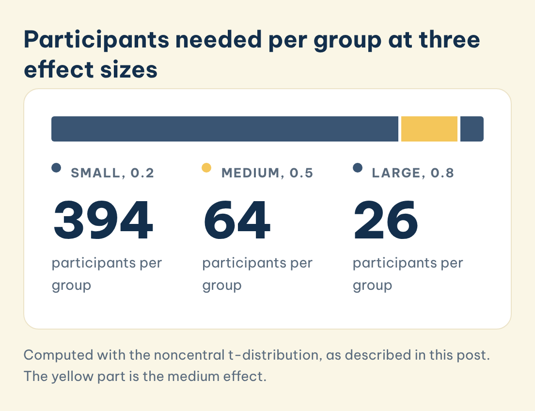
With 26 per group for d = 0.8 against 394 for d = 0.2, the range across the three benchmarks is about 15-fold. Across all six cells of the table, the smallest requirement is 26 per group (d = 0.8, 80% power) and the largest is 651 per group (d = 0.2, 95% power), a spread of 25-fold. Moving from a medium to a small effect multiplies the required sample by more than six (394 against 64 per group at power .80). If you cannot justify a medium effect from the literature, plan for a smaller one, or say openly in your limitations that your study can only detect large differences.
◆ Question 4 / 6 · Paired and one-sample
How does the sample size change for a paired or one-sample t-test?
Direct answer: A paired design usually needs far fewer participants, because each person acts as their own comparison. Using the same checks, a paired effect of dz = 0.5 needs 34 pairs for power .80 and 54 pairs for power .95. Choose the matched pairs option under the t tests family.
For a paired test, G*Power asks for the effect size of the difference scores, usually written dz, not the d you would use for two separate groups, so the two numbers are not interchangeable. We computed the paired figures with the noncentral t-distribution: the exact power is 0.8078 at 34 pairs but 0.7954 at 33, and 0.9502 at 54 pairs against 0.9465 at 53. The same method gives 199 pairs at .80 and 327 at .95 for a dz of 0.2, and 15 pairs at .80 and 23 at .95 for a dz of 0.8. A one-sample t-test uses the same formula, with degrees of freedom equal to n minus 1, so the same effect of 0.5 gives the same 34 and 54 mathematically. In our computation, a paired design at power .80 needs 68 measurements against 128 for the independent version when dz and d are both 0.5, but the two effect sizes are not comparable, so do not use this as a reason to choose a design. Confirm the one-sample number on your own screen. The menu names differ slightly from the independent-samples path, so look for the option that describes matched pairs, or a single sample compared with a fixed value, inside the t tests family. If you are unsure which test fits your data, read Welch's t-test versus Student's t-test before you calculate, and paired t-test reporting in APA style for the paired case.
◆ Question 5 / 6 · Reporting
How do you report a G*Power calculation in your methods section?
Direct answer: State the software and version, the test, the tails, alpha, power, the effect size with its source, and the resulting sample size. Then give the final recruitment target after allowing for dropout. Cite the G*Power paper, as the authors request (Heinrich-Heine-Universität Düsseldorf, n.d.).
A reader should be able to reproduce your number from what you write. A typical sentence (using the figures above) reads: "An a priori power analysis in G*Power 3.1 (Faul et al., 2009) for an independent-samples t-test, two-tailed, with d = 0.5, alpha = .05 and power = .80, indicated a required sample of 128 participants (64 per group)." The authors ask users to cite one or both of two papers (Faul et al., 2007; Faul et al., 2009), and the version number you report should match the one you actually ran. Justify d with a source, such as a previous study or a pilot, and not with the word "medium" alone. Finally, inflate the target for attrition: divide the required number by one minus the expected dropout proportion. With 128 needed and 15% dropout expected, recruit 128 ÷ 0.85, which rounds up to 151 (an extra 23 people, about 18% more). For the paired case, 34 pairs at 15% dropout becomes 40 pairs (34 ÷ 0.85 = 40). A complete report names six settings: the test family (t tests), the number of tails (2), alpha (5%), power (80% or 95%), the effect size with its source, and the allocation ratio, plus the program version, for example 3.1.9.7 on Windows (Heinrich-Heine-Universität Düsseldorf, n.d.). Your reporting of the finished analysis should also include an effect size and interval, as explained in our guide to reporting effect sizes and confidence intervals.
◆ Question 6 / 6 · Getting help
How can MAAS help you plan your sample size?
Direct answer: MAAS works as a mentor and advisor. An expert in the SPSS, R and Python data analysis service can explain each G*Power input, talk through where your effect size comes from, and review your methods paragraph. You run the calculation yourself and write it in your own words.
A mentor can sit with you while you open the program, test how the answer changes when you move d or the allocation ratio, and explain what each change means for your recruitment plan. The mentor guides and reviews. The choices, the calculation and the writing stay with you, which keeps the work yours and leaves you able to defend it at a meeting or viva. Department rules on documenting power analyses come first.
Frequently asked questions
Is the software free?
Yes. Faul et al. (2007) state in their abstract that G*Power 3 is free, and Heinrich-Heine-Universität Düsseldorf (n.d.) hosts the downloads for Windows (3.1.9.7) and Mac (3.1.9.6).
Which menu option do I pick for two independent groups?
Choose "t tests", then "Means: Difference between two independent means (two groups)", and set the analysis to "A priori" (Kang, 2021).
How many participants do I need for a t-test with d = 0.5?
For two independent groups with a two-tailed test, alpha = .05 (5%) and power .80 (80%), you need 64 per group, 128 in total. For a paired design the figure is 34 pairs (dz = 0.5), and 54 pairs at power .95 (95%) (Kang, 2021, for the independent case).
Should I use 0.2, 0.5 or 0.8 as my effect size?
Use values from earlier studies or a pilot where you can. Faul et al. (2007) note that Cohen's small, medium and large conventions may mean different things for different tests.
Does the calculated sample size include dropouts?
No. The number is what you need to analyse. Divide it by one minus the expected dropout proportion to get your recruitment target, for example 128 ÷ 0.85 = 151 at 15% dropout.
Can I run the power analysis after collecting my data?
You can, because G*Power 3 offers post hoc power analysis as one of its analysis types (Faul et al., 2007). But Faul et al. (2007) recommend specifying population effect sizes on a priori grounds rather than taking them from the observed sample, so power computed from your own result tells a marker little. Plan the number before data collection and report that plan (Kang, 2021).
Related guides
References
Cohen, J. (1988). Statistical power analysis for the behavioral sciences (2nd ed.). Lawrence Erlbaum Associates.
Faul, F., Erdfelder, E., Lang, A.-G., & Buchner, A. (2007). G*Power 3: A flexible statistical power analysis program for the social, behavioral, and biomedical sciences. Behavior Research Methods, 39(2), 175-191. https://doi.org/10.3758/BF03193146
Faul, F., Erdfelder, E., Buchner, A., & Lang, A.-G. (2009). Statistical power analyses using G*Power 3.1: Tests for correlation and regression analyses. Behavior Research Methods, 41(4), 1149-1160. https://doi.org/10.3758/BRM.41.4.1149
Heinrich-Heine-Universität Düsseldorf. (n.d.). GPower*. https://www.psychologie.hhu.de/arbeitsgruppen/allgemeine-psychologie-und-arbeitspsychologie/gpower
Kang, H. (2021). Sample size determination and power analysis using the G*Power software. Journal of Educational Evaluation for Health Professions, 18, Article 17. https://doi.org/10.3352/jeehp.2021.18.17
Not sure how this guide applies to your own case? Talk it through with MAAS in a free 20-minute consultation.
Book a free consultation ▸