
◆ Research Methods
What is the Mann-Whitney U test and when should you use it?
Direct answer: The Mann-Whitney U test compares two independent groups when the outcome is ordinal or skewed, so a t-test is a poor fit. It ranks all scores together and asks whether one group tends to hold higher ranks than the other. It is the non-parametric counterpart of the independent-samples t-test.
Last updated: 2026-10-21
Category: research-methods
Students usually meet this test at the moment a histogram looks wrong, whether in a first-year module or in a 2026 dissertation. The marks pile up at one end, or the outcome is a 5-point rating, and the independent-samples t-test no longer feels safe. This guide covers what the Mann-Whitney U test does, how U is built from ranks, how to run it in SPSS and how to report it in APA 7. The general logic of p-values is not repeated here, because the guide on choosing the right statistical test already places this test among its neighbours.
◆ Question 1 / 8 · What is the Mann-Whitney U
What is the Mann-Whitney U test used for?
Direct answer: It tests whether scores in one independent group tend to be higher than scores in another. Because it works on ranks rather than raw values, it suits ordinal data such as ratings, and numerical data that are skewed or contain outliers, where a comparison of means would be distorted by a few extreme scores.
Mann and Whitney (1947) proposed a statistic U that depends on the relative ranks of the observations from two samples, and it is still the standard rank test for two unrelated groups, with 2 samples of sizes n1 and n2 and N = n1 + n2 observations in total. The researcher pools every score, orders them from smallest to largest, and replaces each score with its rank. If the two groups come from the same distribution, the ranks should be shuffled evenly between them. If one group sits higher, its ranks cluster toward the top and U becomes small for the other group.
Mann and Whitney published the test in the Annals of Mathematical Statistics in March 1947, in volume 18, and the SPSS output used by students in 2026 still reports their statistic. Typical uses include comparing satisfaction ratings between 2 cohorts, completion times between 2 interface designs, or exam marks between a taught group and a comparison group when the marks are heavily skewed. In every case the design has one binary grouping variable (such as treatment or control) and one outcome that is ordinal or numerical. McNiven (n.d.), at the University of York, lists the Mann-Whitney U among the options for an ordinal outcome with two groups, and notes that Likert-style items are ordinal, while totals or means built from several items are more commonly treated as scale data.
◆ Question 2 / 8 · When should you use
When should you use Mann-Whitney U instead of a t-test?
Direct answer: Use the Mann-Whitney U when the groups are independent and the outcome is ordinal, or numerical but clearly non-normal with a small sample. Keep the independent-samples t-test when the outcome is roughly normal in each group, because it answers a question about means and uses the raw scores directly.
The two tests answer related but different questions, and the choice should follow the data and the research question rather than the p-value each produces. The table below sets them side by side.
| Feature | Independent-samples t-test | Mann-Whitney U test |
|---|---|---|
| Type | Parametric | Non-parametric (rank-based) |
| Outcome variable | Numerical, roughly normal in each group | Ordinal, or numerical and skewed |
| Groups | Two independent groups | Two independent groups |
| What is compared | Population means | Whether one group tends to score higher |
| Sensitivity to outliers | High | Low, since only ranks are used |
| Typical effect size | Cohen's d | r = z / √N |
Consider a hypothetical module in which 30 students in the 2025 cohort and 28 students in the 2026 cohort rate a workshop on a 5-point scale, from 1 for poor to 5 for excellent. A rating of 4 is not exactly twice a rating of 2, and the 58 ratings are likely to pile up at 4 and 5. The outcome is ordinal and skewed, the cohorts are independent, and so the Mann-Whitney U test is the natural choice. Had the same 58 students reported weekly study hours, a roughly bell-shaped variable, the t-test would be the stronger choice.
A common shortcut says to switch to the Mann-Whitney U whenever a normality test fails. That rule is too blunt. With a large sample, a normality test flags trivial departures, and the t-test is often still reasonable. With a very small sample the test has little power to detect non-normality at all. Examine the histograms and the measurement level first, and decide on those grounds, using the usual 5% significance level only after the choice of test has been made (McNiven, n.d.). The statistics help guide for theses explains how to document that decision so your examiner can follow it.
◆ Question 3 / 8 · What are the hypotheses
What are the hypotheses and assumptions of the test?
Direct answer: The test needs two independent groups and an ordinal or numerical outcome. To describe the result as a difference in medians, the two distributions must also have a similar shape. Without that, a significant result shows only that one group tends to score higher, not that the medians differ.
The assumptions are modest. The two groups must be independent, which means no participant appears in both, and the dependent variable must be ordinal or numerical. Shape is the part students miss. Hart (2001) explains in the BMJ, volume 323, issue 7309, on pages 391 to 393, that the test assumes two samples drawn from populations of the same shape, and that it can detect differences in shape and spread as well as differences in medians. His opening paragraph puts it plainly:
"Whereas a t test is a test of population means, the Mann-Whitney test is commonly regarded as a test of population medians. This is not strictly true, and treating it as such can lead to inadequate analysis of data." (Hart, 2001, p. 391)
For that reason the cautious wording of the hypotheses is: the null hypothesis states that the two populations have the same distribution, and the alternative states that scores in one population tend to be larger than in the other. Mann and Whitney (1947) framed the test as one of whether a random variable is stochastically larger than another. Write "medians" in your hypotheses only after you have looked at the histograms of both groups and found them to be similar in shape and spread.
◆ Question 4 / 8 · How is the U statistic
How is the U statistic calculated?
Direct answer: Rank all scores from both groups together, sum the ranks for each group, then compute U = R minus n(n + 1)/2 for each group. The smaller of the two U values is reported. The two values always add up to n1 multiplied by n2, which gives a quick arithmetic check.
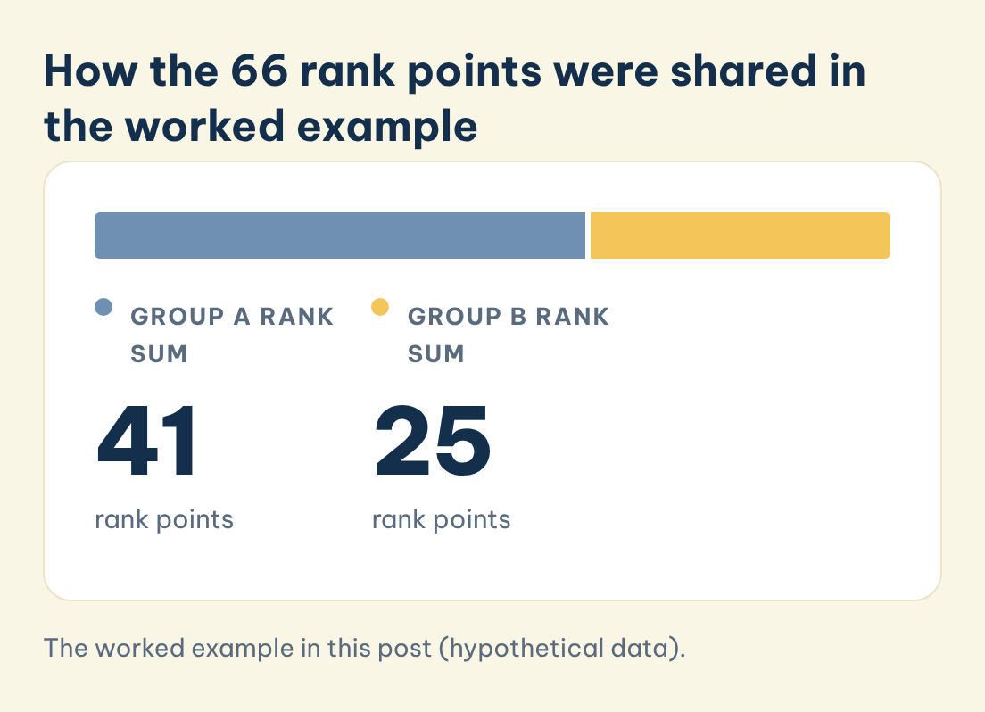
How the 66 rank points were shared in the worked example
Rank sums for the 11 invented scores in this post: group A (5 students) and group B (6 students).
Group A rank sum
41
rank points
Group B rank sum
25
rank points
Save this figure
The following example is hypothetical and uses invented marks. Five students used a new revision method (group A) and six used their usual method (group B). Group A scored 14, 18, 11, 21 and 16. Group B scored 9, 12, 8, 13, 10 and 15.
Pooling the 11 scores and ranking them from the lowest gives: 8 (rank 1), 9 (2), 10 (3), 11 (4), 12 (5), 13 (6), 14 (7), 15 (8), 16 (9), 18 (10) and 21 (11). Group A holds ranks 4, 7, 9, 10 and 11, so its rank sum is R_A = 41. Group B holds ranks 1, 2, 3, 5, 6 and 8, so R_B = 25. As a check, 41 + 25 = 66, which equals 11 × 12 / 2.
Each U comes from the rank sum minus the smallest possible rank sum for that group, the same arithmetic used in the University of Bristol teaching notes listed under Tools & resources. For group A, U_A = 41 − 5 × 6 / 2 = 41 − 15 = 26. For group B, U_B = 25 − 6 × 7 / 2 = 25 − 21 = 4. The check n1 × n2 = 5 × 6 = 30 holds, because 26 + 4 = 30. The reported statistic is the smaller value, U = 4. When scores tie, each tied score receives the average of the ranks it occupies.
With samples this small the exact p-value is the right one to read. The two groups also differ in simple descriptives: group A has a mean of 16.0 and a median of 16, while group B has a mean of about 11.2 and a median of 11, so the gap is 5 marks on the median and about 4.8 on the mean. Among the 462 equally likely ways of assigning 5 of the 11 ranks to group A, exactly 24 give a U of 4 or less in either direction, so the exact two-sided p is 24 / 462 = .052. The normal approximation, with a mean of 15 and a standard deviation of about 5.48, gives z = −2.01 and p = .045. The two routes disagree about significance at .05, which is why SPSS offers an exact option and why Shier (2004) tells readers to look at both the exact and the asymptotic significance.
◆ Question 5 / 8 · How do you run
How do you run the Mann-Whitney U test in SPSS?
Direct answer: Check the measurement level of the outcome in Variable View (Scale or Ordinal as appropriate), then open Analyze, Nonparametric Tests and choose the two-independent-samples procedure. Move the outcome to the test list, define the two group codes, tick Mann-Whitney U and request exact significance when the sample is small.
Menu names depend on the SPSS version. In the older layout the route is Analyze > Nonparametric Tests > Legacy Dialogs > 2 Independent Samples, where you confirm that Mann-Whitney U is selected under Test Type and click Exact if you want exact probabilities (Shier, 2004). In the newer layout the route is Analyze > Nonparametric Tests > Independent Samples, and the procedure may report an exact significance for small samples; check that the output shows an exact p-value and, if it does not, use the legacy dialog with Exact.
Shier (2004) shows a small-sample output of exactly this kind, with U = 3.000, W = 13.000 and z = −1.715, an asymptotic significance of .086 and an exact significance of .111, so the two p-values differ noticeably (.086 against .111) even when both lead to the same decision. The output gives U, the Wilcoxon W (the rank sum of the smaller group), z, the asymptotic significance and, when requested, the exact significance. Compare the significance column with the 5% level (alpha = .05), then copy U, z and the p-value into your results, then compute the effect size by hand or in a spreadsheet, because SPSS does not print it in the basic output. If you want to practise on your own dataset with a tutor beside you, MAAS offers SPSS and Python data analysis guidance that explains your output rather than replacing your analysis.
◆ Question 6 / 8 · How do you report the result
How do you report the result in APA 7 with an effect size?
Direct answer: Report the medians of both groups, U, z, the p-value and an effect size. Fritz et al. (2012) give the conversion r = z / √N, where N is the total number of observations, with benchmarks of .1 for small, .3 for medium and .5 for large.
Fritz et al. (2012) point out that packages such as SPSS print the z value alongside U, and that r can be calculated directly from it. In the worked example, z = −2.01 and N = 11, so r = 2.01 / √11 = .61, a large effect by the usual benchmarks. Drop the sign when quoting r as a magnitude, and state which group scored higher in words. The longer guide on reporting effect sizes and confidence intervals in APA 7 covers the typography of italics, decimals and leading zeros.
Three benchmarks are worth memorising before you write up. Cohen's guidelines treat r = .1 as small, r = .3 as medium and r = .5 as large, as quoted by Fritz et al. (2012). A result of .61 therefore sits above the .5 line for large effects, and a result of .08 would sit below the .1 line. Also state the group sizes, here n = 5 and n = 6, so the reader can judge how much weight a single study with 11 participants can carry.
An APA-style sentence for the hypothetical data would read: a Mann-Whitney U test indicated that the revision-method group (n = 5, Mdn = 16) scored higher than the usual-method group (n = 6, Mdn = 11), U = 4, z = −2.01, exact p = .052, r = .61. Because the exact p exceeds .05, the honest wording is that the difference did not reach significance at the .05 level despite a large observed effect, and that a larger sample would be needed to settle it. Medians are only appropriate here if the two distributions have a similar shape, as discussed above.
◆ Question 7 / 8 · How does the Mann-Whitney U
How does the Mann-Whitney U test differ from Fisher's exact test?
Direct answer: They suit different data. The Mann-Whitney U compares an ordinal or numerical outcome between two groups using ranks. Fisher's exact test analyses a table of counts for two binary categorical variables, typically when expected cell counts are too small for a chi-square test.
Choose by the measurement level of the outcome. If each participant has a score, a rating or a time, the data can be ranked and the Mann-Whitney U applies. If each participant is only classified, for example passed or failed within treatment or control, the data form a two-by-two table of counts, and Fisher's exact test is the small-sample option. The University of York Maths Skills Centre guide lists Fisher's exact test beside the chi-square test for two nominal variables, which is a different branch from the ordinal-outcome branch where the Mann-Whitney U sits (McNiven, n.d.). Reducing a numerical outcome of, say, 40 marks to pass or fail just to use Fisher's test throws information away, so avoid it unless the research question is genuinely about a threshold.
◆ Question 8 / 8 · Why is it called
Why is it called the Mann-Whitney U test?
Direct answer: It carries the names of Henry Mann and Donald Whitney, who published the test in 1947, and the letter U is the name of their statistic. Frank Wilcoxon had proposed an equivalent test in 1945, so the same procedure is also called the Wilcoxon rank-sum test.
Mann and Whitney (1947) wrote that Wilcoxon had proposed an equivalent test in the Biometrics Bulletin in December 1945 but gave only a few points of the distribution of his statistic. Wilcoxon (1945), in the Biometrics Bulletin, introduced comparing groups by ranking methods, and Mann and Whitney supplied the fuller distribution, with tables for samples up to 8 observations per group, and observed that at that point the distribution is almost normal. The 1945 paper (Wilcoxon, 1945) appeared in volume 1, issue 6 of Biometrics Bulletin, and the 1947 paper in volume 18, issue 1 of the Annals of Mathematical Statistics, pages 50 to 60. That history explains why textbooks, journals and software use different labels for what is mathematically the same test. When you meet "Wilcoxon rank-sum" in a paper, read it as the two-sample test described here, and do not confuse it with the Wilcoxon signed-rank test, which is for paired data.
Frequently asked questions
What is the Mann-Whitney U test used for?
This test compares two independent groups when the outcome is ordinal, or numerical but skewed, by ranking all scores together. The question is whether scores in one group tend to be higher than in the other, without assuming a normal distribution (McNiven, n.d.).
When should I use Mann-Whitney U instead of a t-test?
Choose it for independent groups with an ordinal outcome, or a clearly non-normal outcome in a small sample. If your question concerns means and the data look roughly normal, the t-test is still the better tool.
Does the Mann-Whitney U test compare medians?
Only under a condition. Hart (2001) states that treating it as a test of medians is not strictly true. The medians are a fair summary when the two distributions have a similar shape, so check the histograms before you write "medians" (Hart, 2001).
What is the difference between Mann-Whitney U and Fisher's exact test?
Mann-Whitney U ranks an ordinal or numerical outcome across two groups. Fisher's exact test analyses counts in a two-by-two table of categories. The type of outcome decides which one applies (McNiven, n.d.).
Why is it called the Mann-Whitney U test?
The name comes from Henry Mann and Donald Whitney, who published it in 1947. Wilcoxon proposed an equivalent test in 1945, which is why the same procedure is also called the Wilcoxon rank-sum test (Mann & Whitney, 1947).
Which effect size should I report with the Mann-Whitney U test?
Report r = z / √N, using the z value printed by SPSS and the total number of observations. Fritz et al. (2012) give benchmarks of .1, .3 and .5 for small, medium and large effects (Fritz et al., 2012).
Should I read the exact or the asymptotic p-value?
With small samples, read the exact value, because the normal approximation can disagree with it, as it does in the worked example above. With large samples the two values are usually close and the asymptotic one is acceptable (Shier, 2004).
Related reading
- How do you choose the right statistical test?: where the Mann-Whitney U sits among the common tests
- How do you report effect size and confidence intervals in APA 7?: the typography of results sentences
- Thesis statistics help: documenting your choice of test for an examiner
References
Fritz, C. O., Morris, P. E., & Richler, J. J. (2012). Effect size estimates: Current use, calculations, and interpretation. Journal of Experimental Psychology: General, 141(1), 2-18. https://doi.org/10.1037/a0024338
Hart, A. (2001). Mann-Whitney test is not just a test of medians: Differences in spread can be important. BMJ, 323(7309), 391-393. https://doi.org/10.1136/bmj.323.7309.391
Mann, H. B., & Whitney, D. R. (1947). On a test of whether one of two random variables is stochastically larger than the other. The Annals of Mathematical Statistics, 18(1), 50-60. https://doi.org/10.1214/aoms/1177730491
McNiven, G. (n.d.). Which statistical test? University of York Maths Skills Centre. https://subjectguides.york.ac.uk/maths-skills-centre/which-statistical-test
Shier, R. (2004). Statistics: 2.3 The Mann-Whitney U test. statstutor. https://www.statstutor.ac.uk/resources/uploaded/mannwhitney.pdf
Wilcoxon, F. (1945). Individual comparisons by ranking methods. Biometrics Bulletin, 1(6), 80–83. https://doi.org/10.2307/3001968
Tools & resources
- Statstutor. Wilcoxon Mann-Whitney test resources. https://www.statstutor.ac.uk/topics/nonparametric-methods/wilcoxon-mann-whitney-test/
- University of Bristol Centre for Multilevel Modelling. Mann-Whitney tests in SPSS (practical). https://www.bristol.ac.uk/cmm/media/research/ba-teaching-ebooks/pdf/Mann%20Whitney%20-%20Practical.pdf
Not sure how this guide applies to your own case? Talk it through with MAAS in a free 20-minute consultation.
Book a free consultation ▸