
◆ Research Methods
How do you read a chi-square table and run a chi-square test?
A chi-square table lists critical values: you pick the row for your degrees of freedom and the column for your significance level, then compare your test statistic with the number where they meet. If your statistic is larger, the result is significant. The National Institute of Standards and Technology (n.d.-a) publishes the standard table.
◆ Question 1 / 9 · The test
What does a chi-square test actually test?
Direct answer: A chi-square test compares counts you observed with counts you would expect if the null hypothesis were true. There are two common versions: the test of independence asks whether two categorical variables are related, and the goodness-of-fit test asks whether one variable follows a stated distribution.
Sharpe (2015) separates the two by shape: a test of independence works on a contingency table of rows and columns, such as 2 x 2 or larger, while a goodness-of-fit test works on a single set of categories. The National Institute of Standards and Technology (n.d.-b) describes goodness of fit as testing whether sample data came from a population with a specified distribution, with the statistic built from the sum of (observed minus expected) squared, divided by expected, across all categories.
Both versions use the same arithmetic and the same table, and only the degrees of freedom differ. Neither version tells you how strong an association is (McHugh, 2013), which is why an effect size always follows. The test also needs counts of separate people or items, not percentages and not repeated measurements on the same person. If your outcome is a mean rather than a count, you want a different test, and our guide to choosing the right statistical test shows how to decide.
◆ Question 2 / 9 · Degrees of freedom
How do you find the degrees of freedom?
Direct answer: For a test of independence, degrees of freedom equal (rows minus 1) multiplied by (columns minus 1). A 2 x 2 table has 1 df and a 3 x 3 table has 4. For goodness of fit with k categories, the standard rule is k minus 1.
McHugh (2013) gives the independence formula and both examples: "a 2 x 2 table has 1 df. (2-1) x (2-1) = 1. A 3 x 3 table has (3-1) x (3-1) = 4 df." The goodness-of-fit rule of k minus 1 is standard in statistics textbooks.
Degrees of freedom matter because the same statistic means different things at different df. A value of 6.00 is significant at the .05 level with 2 df (cut-off 5.991) but not with 4 df (cut-off 9.488), as the table in the next section shows. Students lose marks here more than anywhere else, usually by counting the categories instead of the table. The 2 x 2 case is the most common in coursework, since it has 1 df and the .05 cut-off of 3.841 from the table below. Count the rows and columns of the table of observed counts, ignore the totals row and column, and apply the formula.
◆ Question 3 / 9 · Reading the table
How do you read a chi-square table?
Direct answer: Find your df in the row labels, find your significance level in the column, and read the critical value where they cross. Reject the null hypothesis when your statistic is greater than that number. Check the column heading carefully, because some tables label columns by 1 minus alpha.
The National Institute of Standards and Technology (n.d.-a) labels its columns "probability less than the critical value", so the .05 level sits under the column headed 0.95 and the .01 level under 0.99. Its instruction for an upper-tail test is to use the column for 1 minus alpha and to reject when the statistic is larger than the tabled value. The values below for 1 to 4 df come from that page.
| df | Critical value at alpha = .05 | Critical value at alpha = .01 |
|---|---|---|
| 1 | 3.841 | 6.635 |
| 2 | 5.991 | 9.210 |
| 3 | 7.815 | 11.345 |
| 4 | 9.488 | 13.277 |
The same page keeps climbing at higher df, with .05 values of 11.070 at 5 df, 12.592 at 6 df and 18.307 at 10 df, so a statistic of 12.35 beats the .05 cut-off at 1 to 5 df but not at 6 df (12.592) or 10 df (18.307). Many searches ask whether a chi-square table is one-tailed or two-tailed. The test is built so that only large statistics count against the null hypothesis, because squaring the differences makes every deviation positive. So you reject in the upper tail, and you do not split alpha between two tails. The test is non-directional about the association: it says there is a relationship, not which way it runs. Some textbooks call this a one-tailed test because only the upper tail is used, even though the hypothesis itself is non-directional.
◆ Question 4 / 9 · Worked example
How do you run a test of independence, step by step?
Direct answer: Build the table of observed counts, calculate the expected count for each cell as row total times column total divided by the grand total, add up (observed minus expected) squared over expected, then compare the sum with the critical value for your df (National Institute of Standards and Technology, n.d.-b).
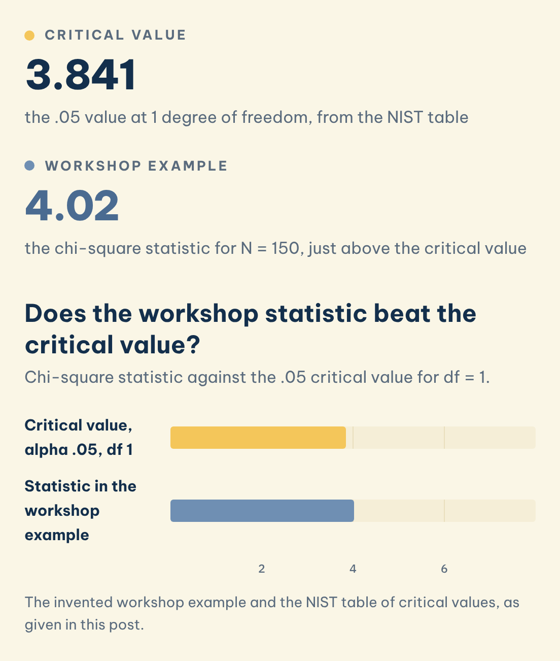
Critical value
3.841
the .05 value at 1 degree of freedom, from the NIST table
Workshop example
4.02
the chi-square statistic for N = 150, just above the critical value
Does the workshop statistic beat the critical value?
Chi-square statistic against the .05 critical value for df = 1.
Save this figure
Take an invented example. A tutor asks 150 students whether they attended a statistics workshop and whether they handed in their report on time. Of 80 students who attended, 54 were on time and 26 late. Of 70 who did not attend, 36 were on time and 34 late. The row totals are 80 and 70, the column totals are 90 on time and 60 late, and N = 150.
| Expected count | On time | Late |
|---|---|---|
| Attended (80) | 80 x 90 / 150 = 48 | 80 x 60 / 150 = 32 |
| Did not attend (70) | 70 x 90 / 150 = 42 | 70 x 60 / 150 = 28 |
The statistic follows the definition given by the National Institute of Standards and Technology (n.d.-b), and an alpha of .05 means accepting a 5% risk of rejecting a null hypothesis that is true. Each cell then contributes its squared gap divided by its expected count. The gaps are all 6 in size, so the four contributions are 36/48 = 0.75, 36/32 = 1.125, 36/42 = 0.857 and 36/28 = 1.286. Their sum is 4.02, and with df = 1 the critical value at .05 is 3.841, so 4.02 exceeds it. The result is significant at .05 but below 6.635, so p falls between .01 and .05. Software gives p = .045. This is the plain Pearson test without a continuity correction.
◆ Question 5 / 9 · Goodness of fit
How is a goodness-of-fit test different?
Direct answer: A goodness-of-fit test starts from one set of counts and a stated expectation, such as equal shares, and compares them. Degrees of freedom are the number of categories minus 1. The table lookup and the decision rule are the same as for a test of independence (National Institute of Standards and Technology, n.d.-a).
Following the same definition from the National Institute of Standards and Technology (n.d.-b), suppose 90 students each choose one of three seminar slots and you expected an even split of 30 per slot. You observe 40, 30 and 20. The contributions are (40 - 30) squared over 30 = 3.333, 0 for the middle slot, and (20 - 30) squared over 30 = 3.333, so the statistic is 6.67. With 3 categories df = 2, and the .05 critical value is 5.991 from the table above. Because 6.67 is larger, the observed pattern differs from an even split. It is also below 9.210, so p lies between .01 and .05, and software gives p = .036.
The expected shares do not have to be equal. They can come from a theory or a known population, for example a national age breakdown, and then each expected count is the share multiplied by your total. The one rule is that the expected counts must add up to your total.
◆ Question 6 / 9 · p value
Can you get the p value from the table, or do you need software?
Direct answer: A table only brackets p: it tells you whether p is above or below .05 and .01. Software gives the exact value, which APA Style asks you to report (American Psychological Association, n.d.). The decision to reject is the same either way, and the two will never disagree for the same alpha.
Software such as SPSS, R or Python reports exact values. Using a table, you can say "p < .05" when the statistic beats the .05 column and "p < .01" when it beats the .01 column, and nothing sharper than that. American Psychological Association (n.d.) asks for exact p values to two or three decimals, with p < .001 for anything smaller, so the exact figure from SPSS, R, Python or a spreadsheet function is what belongs in your report. Many searches also ask about calculators, and they all do the same job: they take your statistic and df and return the area in the upper tail.
Use the table to check the software, since a printed table cannot hide a data-entry slip, and the two numbers should agree to the bracket. If you run the test on raw data in SPSS or Python, the output shows the chi-square, df and p together, and you only need to copy them accurately. Our data analysis support for assignments helps you read that output and explain it.
◆ Question 7 / 9 · Assumptions
What are the assumptions, and when should you use Fisher's exact test?
Direct answer: Observations must be independent, counts must be raw frequencies, and expected counts must be large enough. A common working rule is that no more than 20% of cells have an expected count below 5 and none below 1 (Sharpe, 2015). When this fails, especially in a 2 x 2 table, Fisher's exact test is the usual alternative.
Sharpe (2015) traces the working rule to Cochran, writing that he "recommended instead a set of working rules such that no cells should have an expected frequency less than one and no more than 20% of cells should be between one and five" (p. 8, by PDF page numbering because the article carries no printed page range). McHugh (2013) adds that the study groups must be independent, so paired or repeated data cannot use the test. McHugh (2013) also states the same idea as expected counts of 5 or more in at least 80% of cells with none below 1, and says it is most likely to be met when the sample size equals at least the number of cells multiplied by 5. A 2 x 2 table has 4 cells, so 20 observations is the floor. In the workshop example the smallest expected count is 28 and N is 150, so both rules are met comfortably.
Roughly 20% of cells below 5 is the most that the working rule allows. If your table fails, you can merge sparse categories where that makes sense, collect more data, or switch to an exact test, since the chi-square p value is an approximation that works poorly with small expected counts. Fisher's exact test uses exact probabilities and is usually the choice for a small 2 x 2 table, and a separate guide will cover it. Planning your numbers before data collection avoids the problem, as shown in our guide to calculating sample size.
◆ Question 8 / 9 · Effect and APA
How big is the effect, and how do you report it in APA 7?
Direct answer: A significant chi-square only says an association exists. Add phi for a 2 x 2 table or Cramér's V for larger ones, then report the statistic as χ²(df, N = sample size) = value, p = exact value. Round the chi-square to two decimals and do not use commas in the degrees of freedom (American Psychological Association, n.d.).
McHugh (2013) states that the chi-square "is a significance statistic, and should be followed with a strength statistic", with Cramér's V as the most common choice, and she warns that V tends to be low even when the result is highly significant. Her own example is a 3 x 2 table with N = 184, a chi-square of 12.35 at 2 df and V = .26. Sharpe (2015) notes that V is identical to phi for a 2 x 2 table, and that Cohen's guideline values of .10, .30 and .50 correspond to small, medium and large for phi. For a 2 x 2 table, phi is the square root of the chi-square divided by N. In the workshop example, 4.02 / 150 = 0.0268, whose square root is .16, a small to medium effect.
For larger tables, V is the square root of the chi-square divided by N times the smaller of (rows minus 1) and (columns minus 1). The University of Southampton Library (n.d.) lists what a report needs: the test statistic, degrees of freedom, sample size, p value and an interpretation. American Psychological Association (n.d.) asks you to italicise Latin symbols such as N and p. Our workshop result is written as: χ²(1, N = 150) = 4.02, p = .045, φ = .16. In words, students who attended the workshop were somewhat more likely to hand in on time. For more on interpreting size, see our guide to reporting effect size and confidence intervals.
◆ Question 9 / 9 · MAAS
How can MAAS help with chi-square tests?
Direct answer: MAAS works as a tutor and advisor. A MAAS expert can walk you through choosing the test, checking assumptions and reading your output, and you run the analysis and write up the findings yourself. The first conversation is free, and prices are set by the scope of your data work.
If your table fails the expected-count rule, or you cannot tell whether your design needs a test of independence or goodness of fit, that is a good moment to talk to someone. Data and analysis support from MAAS starts from your dataset and your question. Bring your coding scheme, your output and your marker's brief, so the conversation can start from what you already have.
Frequently asked questions
Is a chi-square table one-tailed or two-tailed?
The test rejects only in the upper tail, so you compare your statistic with the critical value from the 1 minus alpha column. The National Institute of Standards and Technology (n.d.-a) gives this instruction for upper-tail tests.
What is the critical value of chi-square at .05 with 1 degree of freedom?
It is 3.841, and at .01 it is 6.635. The National Institute of Standards and Technology (n.d.-a) lists these values in its table of critical values.
How do I get a p value from a chi-square table?
You can only bracket it, for example p < .05 or p < .01. For the exact value, use software, because American Psychological Association (n.d.) asks for exact p values to two or three decimals.
What do I do if an expected count is below 5?
Check whether more than 20% of cells fall below 5, or any cell falls below 1. Sharpe (2015) describes this as Cochran's working rule. If it fails, merge categories, collect more data or use Fisher's exact test.
How do I report a chi-square test in APA 7?
Write χ²(df, N = sample size) = value, p = exact value, for example χ²(1, N = 150) = 4.02, p = .045, then add an effect size. The University of Southampton Library (n.d.) lists the elements to include.
Which effect size goes with a chi-square test?
Use phi for a 2 x 2 table and Cramér's V for larger tables. McHugh (2013) describes V as the most common strength statistic to report alongside a significant chi-square.
References
American Psychological Association. (n.d.). Number and statistics guide, APA Style 7th edition. https://apastyle.apa.org/instructional-aids/numbers-statistics-guide.pdf
McHugh, M. L. (2013). The chi-square test of independence. Biochemia Medica, 23(2), 143-149. https://doi.org/10.11613/BM.2013.018
National Institute of Standards and Technology. (n.d.-a). 1.3.6.7.4. Critical values of the chi-square distribution. In NIST/SEMATECH e-handbook of statistical methods. https://www.itl.nist.gov/div898/handbook/eda/section3/eda3674.htm
National Institute of Standards and Technology. (n.d.-b). 1.3.5.15. Chi-square goodness-of-fit test. In NIST/SEMATECH e-handbook of statistical methods. https://www.itl.nist.gov/div898/handbook/eda/section3/eda35f.htm
Sharpe, D. (2015). Your chi-square test is statistically significant: Now what? Practical Assessment, Research, and Evaluation, 20(8), Article 8. https://doi.org/10.7275/tbfa-x148
University of Southampton Library. (n.d.). Reporting your statistics. LibGuides@Southampton. https://library.soton.ac.uk/reporting-your-statistics
Tools & resources
- NIST/SEMATECH e-handbook: critical values of the chi-square distribution (National Institute of Standards and Technology)
- APA Style number and statistics guide (American Psychological Association)
Not sure how this guide applies to your own case? Talk it through with MAAS in a free 20-minute consultation.
Book a free consultation ▸