
◆ Research Methods
What is Bayesian statistics, explained simply for students?
Bayesian statistics is a way of analysing data in which what you already know about a quantity is updated by what your data show. van de Schoot et al. (2021) describe it as an approach based on Bayes' theorem. Its answers come in the form students often wish for: a probability that a hypothesis or a parameter value is true, given the data.
Most undergraduate and master's courses teach only the frequentist route, with p values and confidence intervals, so the Bayesian vocabulary of priors, posteriors and Bayes factors can feel like a different language. This guide explains the core ideas with one worked example, compares credible and confidence intervals, shows how to read a Bayes factor, names two free tools, and points to the checklists that tell you what to report.
◆ Question 1 / 9 · What it is
What is Bayesian statistics in simple terms?
Direct answer: Bayesian statistics is an approach to data analysis in which available knowledge about a parameter is updated with the information in observed data. The starting knowledge is called the prior, the data enter through the likelihood, and the updated result is the posterior distribution (van de Schoot et al., 2021).
The abstract of the Nature Reviews Methods Primers article puts it in one sentence: "Bayesian statistics is an approach to data analysis based on Bayes' theorem, where available knowledge about parameters in a statistical model is updated with the information in observed data" (van de Schoot et al., 2021, p. 1). The article was published in 2021 and has Andrew Gelman and Sarah Depaoli among its eleven authors. A useful picture is a learner who holds a belief, sees evidence, and adjusts the belief by an amount that depends on how strong the evidence is. The Open University (n.d.) offers a free OpenLearn course on the topic, which makes it a sensible companion to this guide.
◆ Question 2 / 9 · Bayes' theorem
How does Bayes' theorem work, with an example?
Direct answer: Bayes' theorem turns the probability of the data given a hypothesis into the probability of the hypothesis given the data. In a screening example with 1% prevalence, 90% sensitivity and a 9% false-positive rate, a positive test means only about a 9.2% chance of disease.
The numbers below are an illustration worked out by the author of this guide, not results from a published study. Imagine a condition that affects 1 person in 100. A test detects it in 90% of people who have it and wrongly flags 9% of people who do not. Out of 10,000 people, 100 have the condition and 90 of them test positive, while 9,900 do not have it and 891 of them test positive anyway. That makes 981 positives, of whom only 90 are truly ill, so the probability of disease after a positive test is 90 divided by 981, about 9.2%. Most people expect an answer near 90%, because they ignore how rare the condition is to begin with. That starting rarity is the prior, and the 90% and 9% figures are the likelihood. The same calculation in odds form multiplies prior odds of 1 to 99 by a likelihood ratio of 10 to reach posterior odds of 10 to 99.
| Step | Quantity | Value in this illustration |
|---|---|---|
| Prior | Probability of disease before testing | 1% (1 in 100) |
| Likelihood | Positive test if ill / if not ill | 90% / 9% |
| Evidence | Share of all people who test positive | 9.81% |
| Posterior | Probability of disease after a positive test | About 9.2% |
◆ Question 3 / 9 · Prior to posterior
What are the prior, the likelihood and the posterior?
Direct answer: The prior summarises beliefs about a parameter before the data are seen, the likelihood summarises what the data say about it, and the posterior is what is known after combining them. The Open University (n.d.) describes these three parts in its Bayesian statistics course.
The Open University (n.d.) writes that the prior distribution summarises beliefs about the value of a parameter before data are observed, the likelihood function summarises information contained in observed data, and the posterior distribution represents what is known about a parameter after the data have been observed. In the medical example the prior was a single number, but in a dissertation it is usually a whole distribution, for instance a bell-shaped curve centred on a plausible effect size. Fornacon-Wood et al. (2022) make a broadly similar point in plain language: a strong prior formed from earlier evidence means the data must be highly convincing to change it, while an uninformative prior lets the data drive the inference. Because the prior is a choice, you must justify it and show how sensitive your conclusions are to it.
◆ Question 4 / 9 · Credible intervals
What is the difference between a credible interval and a confidence interval?
Direct answer: A 95% credible interval is the range that has a 95% probability of containing the true parameter value, given the data and the prior. A 95% confidence interval instead describes a long-run property of the procedure: across repeated experiments, 95% of such intervals would contain the true value (Fornacon-Wood et al., 2022).
van Doorn et al. (2021, p. 820) state that a credible interval has "a x% probability that the true parameter lies in the interval that ranges from L to U", and they add that this reading is often wrongly attributed to frequentist confidence intervals. That wrong attribution is common in student reports, so it is worth checking your own wording. The credible interval is conditional on the model and the prior. In their worked example, van Doorn et al. (2021) add the condition that the 95% statement holds "assuming that the alternative hypothesis we specify is true", and suggest presenting the unconditional posterior if you do not want to make that assumption. The width of the interval and the reporting rule matter too: Kruschke (2021, p. 1286) notes that 95% is a conventional probability mass, but whatever mass you choose must be clearly reported. In practice, quote the posterior median or mean together with the interval and say which mass you used.
◆ Question 5 / 9 · Bayes factors
What is a Bayes factor and how do you read it?
Direct answer: A Bayes factor compares how well two hypotheses predict the data. BF10 above 1 favours the alternative and BF10 below 1 favours the null. van Doorn et al. (2021) call a Bayes factor of 1 to 3 weak, 3 to 10 moderate and above 10 strong evidence, but these labels are rules of thumb.
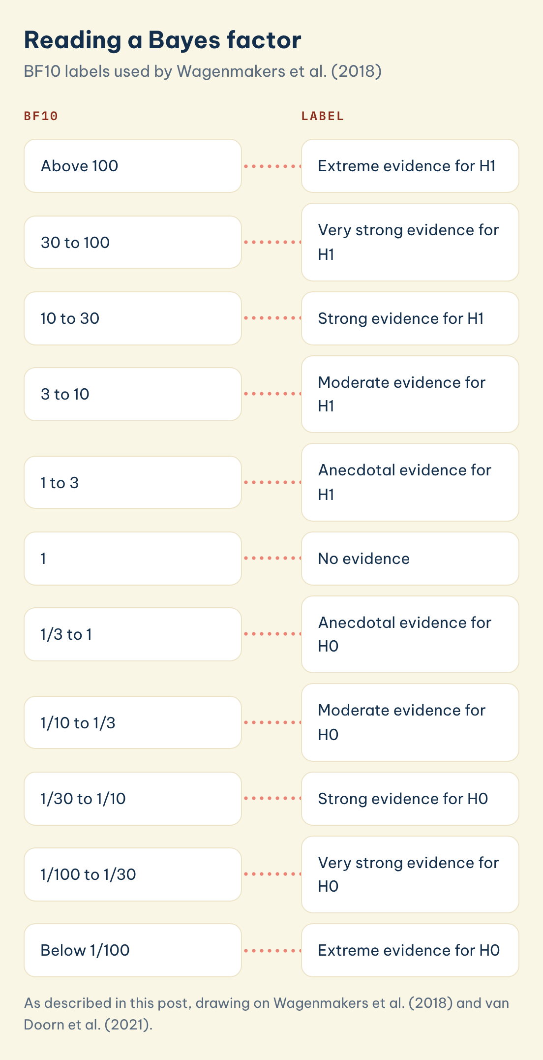
Wagenmakers et al. (2018) reproduce a table that Lee and Wagenmakers adapted from Jeffreys, so the scale is cited here as cited in Wagenmakers et al. (2018). It runs from extreme evidence for H1 when BF10 exceeds 100 down to extreme evidence for H0 when BF10 is below 1/100. van Doorn et al. (2021) use a coarser three-band version and stress that the classifications "should only be used as general rules of thumb to facilitate communication and interpretation of evidential strength" (van Doorn et al., 2021, p. 820). Wagenmakers et al. (2018, p. 67) make the same point by paraphrasing a well-known line by Rosnow and Rosenthal about p values: "surely, God loves the Bayes factor of 2.5 nearly as much as he loves the Bayes factor of 3.5." Note also that a Bayes factor is not the probability that the hypothesis is true. In the medical illustration a likelihood ratio of 10 still left the posterior near 9.2%.
| BF10 | Label used by Wagenmakers et al. (2018) |
|---|---|
| Above 100 | Extreme evidence for H1 |
| 30 to 100 | Very strong evidence for H1 |
| 10 to 30 | Strong evidence for H1 |
| 3 to 10 | Moderate evidence for H1 |
| 1 to 3 | Anecdotal evidence for H1 |
| 1 | No evidence |
| 1/3 to 1 | Anecdotal evidence for H0 |
| 1/10 to 1/3 | Moderate evidence for H0 |
| 1/30 to 1/10 | Strong evidence for H0 |
| 1/100 to 1/30 | Very strong evidence for H0 |
| Below 1/100 | Extreme evidence for H0 |
Reading a Bayes factor
BF10 labels used by Wagenmakers et al. (2018)
BF10
Label
Above 100
Extreme evidence for H1
30 to 100
Very strong evidence for H1
10 to 30
Strong evidence for H1
3 to 10
Moderate evidence for H1
1 to 3
Anecdotal evidence for H1
1
No evidence
1/3 to 1
Anecdotal evidence for H0
1/10 to 1/3
Moderate evidence for H0
1/30 to 1/10
Strong evidence for H0
1/100 to 1/30
Very strong evidence for H0
Below 1/100
Extreme evidence for H0
Save this figure
◆ Question 6 / 9 · Bayesian or frequentist
How is Bayesian statistics different from frequentist statistics?
Direct answer: Frequentist methods treat parameters as fixed and judge a procedure by what would happen over many repetitions, while Bayesian methods treat the parameter as uncertain and describe that uncertainty with a probability distribution. Bayesian analysis therefore needs a prior, which frequentist analysis does not.
Fornacon-Wood et al. (2022) describe frequentist statistics as long-run: a 95% confidence interval tells us that if we repeated the experiment over and over, 95% of the computed intervals would contain the true mean. The Bayesian answer is direct, a probability for the parameter given the data you actually collected. The price is the prior, which must be chosen and defended. Neither approach is automatically better. No source reviewed for this guide tells students when to choose a Bayesian analysis for a dissertation, so treat that as a decision to take with your supervisor, and check your module handbook, because many marking schemes and ethics or methods committees expect a frequentist analysis unless you agree otherwise. If your question is simply whether an effect exists, our guide to hypothesis testing step by step covers the frequentist route, and what statistically significant means shows how to report it.
◆ Question 7 / 9 · Software
Which software can students use for Bayesian analysis?
Direct answer: JASP is a free, open-source program with a graphical interface that offers Bayesian and frequentist versions of the t test, ANOVA and regression. For code-based work, brms is an R package for fitting Bayesian multilevel models using the Stan language (Bürkner, 2017; van Doorn et al., 2021).
van Doorn et al. (2021) introduce JASP as open-source software with a graphical user interface that features both Bayesian and frequentist versions of common tools, which lets you run a Bayesian t test with a few clicks and compare it with the familiar output. Their guidelines are organised in four stages, planning, executing, interpreting and reporting, and their worked example uses a published stereogram dataset. When your model has nested or repeated data, Bürkner (2017) describes brms as an R package for Bayesian multilevel models using Stan. This guide has not tested either program on your data, so run the examples shipped with the software before using it on a real project. If you are weighing it against a classical analysis, the guide to effect sizes and confidence intervals is a useful comparison point.
◆ Question 8 / 9 · Reporting
How do you report a Bayesian analysis?
Direct answer: Report the model, the prior with its justification, the computation details, the posterior summary with a credible interval, any decision criteria, a sensitivity analysis, and how others can reproduce the work. Kruschke (2021) sets these out as Bayesian Analysis Reporting Guidelines, and van de Schoot et al. (2021) update the WAMBS checklist.
Reporting is where many Bayesian papers fall short. Kruschke (2021, p. 1282) cites an extensive review of applied Bayesian analyses in which "55.6% out of 99 articles did not report the hyperparameters specified for the prior, 56.6% did not report checking for chain convergence, and 87.9% did not conduct a sensitivity analysis on the impact of priors." The BARG he proposes has six ordered steps: explain the model, report computation details, describe the posterior distribution, report decisions and their criteria, report a sensitivity analysis, and make the work reproducible. Depaoli and van de Schoot (2017) offer the WAMBS checklist of 10 main points to check, grouped into four stages that run from before estimation to what to do after interpreting the results. For a dissertation, quote the Bayes factor with its subscript (BF10 or BF01) and give the posterior median with a credible interval of stated mass (for example 95%), as van Doorn et al. (2021) recommend.
◆ Question 9 / 9 · A second check
Can MAAS help you check your Bayesian analysis?
Learning to run and interpret a Bayesian analysis yourself is the best preparation for explaining it at a viva. Where a second pair of eyes helps is in choosing between a Bayesian and a frequentist approach, justifying a prior, checking convergence, and making sure the write-up matches the output. Through SPSS, R and Python data analysis support at MAAS, you work alongside a MAAS expert who explains each step of the analysis and reviews how you report it, with you making the decisions about your own project. Bring your research question, your dataset and your university's reporting guidance to the first conversation.
Frequently asked questions
What is Bayes' theorem in simple words?
It is a rule for updating a probability when new evidence arrives. You start from a prior, weigh it by how likely the evidence is under each possibility, and end with a posterior (van de Schoot et al., 2021).
What is a prior in Bayesian statistics?
A prior is the distribution that summarises beliefs about a parameter before the data are observed (The Open University, n.d.). It should be justified and tested for sensitivity.
Is a Bayes factor the same as a p value?
No. A Bayes factor compares two hypotheses, while a p value is computed assuming the null hypothesis is true. A Bayes factor of 3 gives some support but does not warrant confident all-or-none acceptance (van Doorn et al., 2021).
What is a credible interval?
It is a range with a stated probability, such as 95%, of containing the true parameter given the data and prior (Fornacon-Wood et al., 2022).
How difficult is Bayesian statistics?
The core idea, updating a belief with data, is no harder than the logic of a medical test. The harder parts for students are justifying a prior and checking that the model has converged, and the WAMBS checklist sets out 10 points to check so that priors, convergence and reporting are not mishandled (Depaoli & van de Schoot, 2017).
Which free software runs Bayesian analysis?
JASP offers a point-and-click route, and the R package brms suits code-based multilevel models (Bürkner, 2017; van Doorn et al., 2021).
What should I report in a Bayesian dissertation?
Report the prior and its justification, convergence checks, the posterior with a credible interval and a sensitivity analysis, following Kruschke (2021) and the WAMBS checklist (Depaoli & van de Schoot, 2017).
References
Bürkner, P.-C. (2017). brms: An R package for Bayesian multilevel models using Stan. Journal of Statistical Software, 80(1). https://doi.org/10.18637/jss.v080.i01
Depaoli, S., & van de Schoot, R. (2017). Improving transparency and replication in Bayesian statistics: The WAMBS-checklist. Psychological Methods, 22(2), 240–261. https://doi.org/10.1037/met0000065
Fornacon-Wood, I., Mistry, H., Johnson-Hart, C., Faivre-Finn, C., O'Connor, J. P. B., & Price, G. J. (2022). Understanding the differences between Bayesian and frequentist statistics. International Journal of Radiation Oncology*Biology*Physics, 112(5), 1076–1082. https://doi.org/10.1016/j.ijrobp.2021.12.011
Kruschke, J. K. (2021). Bayesian analysis reporting guidelines. Nature Human Behaviour, 5(10), 1282–1291. https://doi.org/10.1038/s41562-021-01177-7
The Open University. (n.d.). Bayesian statistics [Free course]. OpenLearn. https://www.open.edu/openlearn/science-maths-technology/bayesian-statistics/content-section-0?intro=1
van de Schoot, R., Depaoli, S., King, R., Kramer, B., Märtens, K., Tadesse, M. G., Vannucci, M., Gelman, A., Veen, D., Willemsen, J., & Yau, C. (2021). Bayesian statistics and modelling. Nature Reviews Methods Primers, 1, Article 1. https://doi.org/10.1038/s43586-020-00001-2
van Doorn, J., van den Bergh, D., Böhm, U., Dablander, F., Derks, K., Draws, T., Etz, A., Evans, N. J., Gronau, Q. F., Haaf, J. M., Hinne, M., Kucharský, S., Ly, A., Marsman, M., Matzke, D., Gupta, A. R. K. N., Sarafoglou, A., Stefan, A., Voelkel, J. G., & Wagenmakers, E.-J. (2021). The JASP guidelines for conducting and reporting a Bayesian analysis. Psychonomic Bulletin & Review, 28(3), 813–826. https://doi.org/10.3758/s13423-020-01798-5
Wagenmakers, E.-J., Love, J., Marsman, M., Jamil, T., Ly, A., Verhagen, J., Selker, R., Gronau, Q. F., Dropmann, D., Boutin, B., Meerhoff, F., Knight, P., Raj, A., van Kesteren, E.-J., van Doorn, J., Šmíra, M., Epskamp, S., Etz, A., Matzke, D., ... Morey, R. D. (2018). Bayesian inference for psychology. Part II: Example applications with JASP. Psychonomic Bulletin & Review, 25(1), 58–76. https://doi.org/10.3758/s13423-017-1323-7
Not sure how this guide applies to your own case? Talk it through with MAAS in a free 20-minute consultation.
Book a free consultation ▸