
◆ Research Methods
What do left and right skewed distributions tell you?
A skewed distribution is one whose two halves are not mirror images, because one tail stretches further than the other. The direction of that long tail gives the skew its name, and the size of the skew decides how you summarise the data and which tests you can trust in a dissertation.
This guide covers what skew means, how it differs from a normal distribution, how to tell whether your own data are skewed, what the skewness coefficient measures, and how the mean, median and mode usually behave. The MAAS guide to statistics help for a thesis explains how checks like this fit into the wider analysis.
◆ Question 1 / 8 · What skew means
What is meant by a skewed distribution?
Direct answer: A skewed distribution is one that lacks symmetry, so its left and right halves do not look the same around the centre (NIST/SEMATECH, n.d.-a). Right skew, also called positive skew, has the long tail on the right. Left skew, or negative skew, has the long tail on the left.
The NIST engineering statistics handbook defines skewness as "a measure of symmetry, or more precisely, the lack of symmetry", and it calls a data set symmetric "if it looks the same to the left and right of the center point" (NIST/SEMATECH, n.d.-a). Its companion page on histograms adds that in a skewed distribution "it is quite common to have one tail of the distribution considerably longer or drawn out relative to the other tail" (NIST/SEMATECH, n.d.-b).
Students often reverse the labels, because the bulk of a right skewed histogram sits on the left. Kim (2013) puts the rule in a form worth memorising: "A positive skew value indicates that the tail on the right side of the distribution is longer than the left side and the bulk of the values lie to the left of the mean" (Kim, 2013, p. 52). A negative skew value means the reverse, with the long tail on the left and most values to the right of the mean.
◆ Question 2 / 8 · Normal vs skewed
What is the difference between a normal distribution and a skewed distribution?
Direct answer: A normal distribution is symmetric and bell shaped, so its skewness is zero and its mean, median and mode coincide. A skewed distribution has a skewness above or below zero and one stretched tail, so the three measures of centre separate and the mean is no longer a safe summary of a typical value.
| Feature | Normal distribution | Right (positive) skew | Left (negative) skew |
|---|---|---|---|
| Shape | Symmetric bell | Long tail to the right | Long tail to the left |
| Skewness value | 0 | Above 0 | Below 0 |
| Bulk of values | Around the centre | On the left, below the mean | On the right, above the mean |
| Usual order of centre (lowest to highest) | Mean = median = mode | Mode, then median, then mean | Mean, then median, then mode |
| Typical summary | Mean and standard deviation | Median and interquartile range | Median and interquartile range |
NIST/SEMATECH (n.d.-a) states that the skewness for a normal distribution is zero and that any symmetric data should have a skewness near zero. Mishra et al. (2019) add the practical link to centre: if the mean, median and mode coincide, the distribution is called symmetric. The order shown for skewed data is the usual textbook pattern, and the next sections explain when it breaks.
For a symmetric distribution the idea of a typical value is unambiguous. NIST/SEMATECH (n.d.-b) warns that for a skewed distribution "there is no 'center' in the usual sense of the word", and it suggests reporting at least the mean and the median rather than one number alone.
◆ Question 3 / 8 · Spotting skew
How do you know if your data are skewed?
Direct answer: Combine a picture with a number. Draw a histogram, box plot or Q-Q plot, then read the skewness statistic and its standard error from your software. In SPSS these sit under Analyze, Descriptive Statistics, Explore (Kim, 2013). Dividing skewness by its standard error gives a z-score to judge by sample size.
Kim (2013) sets the cut-offs by sample size, because standard errors shrink as samples grow and a z-test then flags trivial departures in large samples:
| Sample size | Rule for skewness | Source |
|---|---|---|
| Under 50 | Non-normal if the absolute z-score is above 1.96 | Kim (2013) |
| 50 to 300 | Non-normal if the absolute z-score is above 3.29 | Kim (2013) |
| Over 300 | Use the histogram and the raw value: an absolute skew above 2 signals substantial non-normality | Kim (2013), citing West et al. |
Mishra et al. (2019) also describe a looser rule of thumb, treating a distribution as approximately normal when skewness or excess kurtosis lies between −1 and +1, and they note that it is less reliable for samples under 300. Their paper describes Q-Q plots, P-P plots and box plots as the visual partners to these numbers.
How to judge skewness by sample size
Cut-offs for the skewness statistic, from Kim (2013)
Sample size
Treat the variable as non-normal when
Under 50
Absolute z above 1.96
50 to 300
Absolute z above 3.29
Over 300
Absolute skew above 2, read with the histogram
Any size, rough guide
Skewness outside -1 to +1 (Mishra et al., 2019)
Save this figure
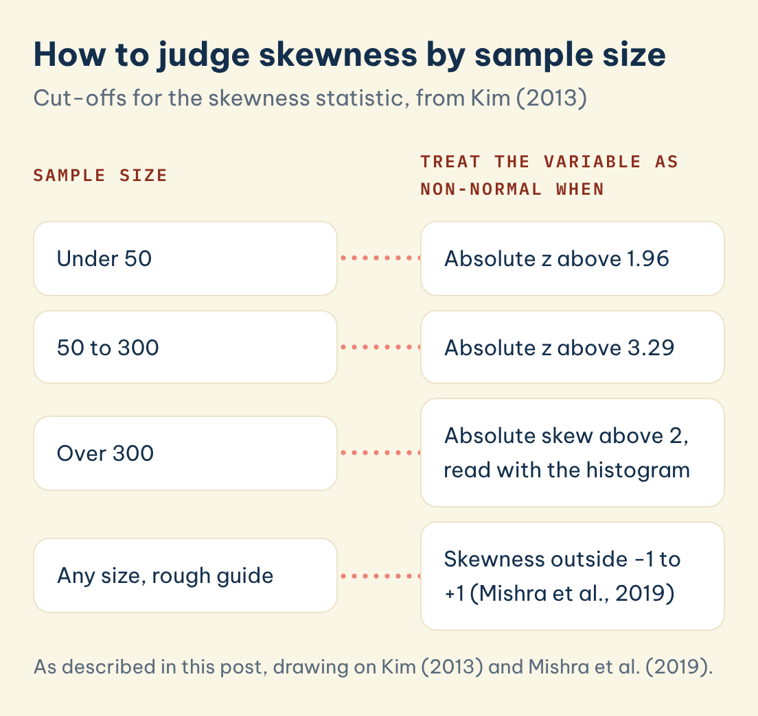
Report what you checked and which rule you used. A sentence that gives the skewness value, its standard error and the decision you took lets a marker follow your reasoning, which matters more than the exact cut-off.
◆ Question 4 / 8 · Positive skew examples
Which distributions are positively skewed?
Direct answer: Variables with a floor but no firm ceiling are often positively skewed. NIST/SEMATECH (n.d.-a) gives failure times in reliability studies, which cannot be negative. In student research the same pattern often appears in income, reaction times, hospital stays and counts of events, where most cases are small and a few are very large.
The mechanism is the lower bound. When values cannot fall below zero but can rise a long way, most observations cluster near the floor and the rare large ones drag the right tail out. NIST/SEMATECH (n.d.-a) notes that "some measurements have a lower bound and are skewed right", and that multi-modal data can affect the sign of the skewness.
Left skew is the mirror case, with a ceiling instead of a floor. Scores on an easy test, where most students reach close to full marks and a few score low, are a common teaching example. Whichever direction you find, check whether the skew reflects the real population or a handful of data entry errors before you decide how to analyse it.
◆ Question 5 / 8 · Mean, median, mode
How do the mean, median and mode behave in a skewed distribution?
Direct answer: The textbook rule says the mean is pulled furthest into the long tail, so under right skew the mean usually sits above the median and the mode sits lowest. Von Hippel (2005) shows that this rule fails surprisingly often, especially in discrete data, so check the actual values.
Von Hippel (2005) found that 14 of the 18 introductory data analysis textbooks he examined teach the rule of thumb relating skew to the positions of the median and mean. His abstract states that the rule "can fail in multimodal distributions, or in distributions where one tail is long but the other is heavy", and that it fails most commonly in discrete distributions where the areas to the left and right of the median are not equal (von Hippel, 2005).
For your dissertation the lesson is practical. Report the mean, median and skewness together for any variable you suspect is skewed, and let the numbers, not a memorised diagram, tell you which way the data lean. Where the mean and median differ a lot, the median and interquartile range usually describe a typical case more honestly.
◆ Question 6 / 8 · Skewness formula
What is the formula for skewness?
Direct answer: The Fisher-Pearson coefficient of skewness averages the cubed deviations from the mean and divides by the standard deviation cubed (NIST/SEMATECH, n.d.-a). Cubing keeps the sign, so long right tails give positive values. Many programs report an adjusted version that corrects for small samples.
In words, the coefficient is g1 = [Σ(Yi − Ȳ)³ / N] / s³, where Ȳ is the mean, s is the standard deviation computed with N in the denominator, and N is the number of data points (NIST/SEMATECH, n.d.-a). The adjusted coefficient multiplies g1 by √[N(N − 1)] / (N − 2), and NIST lists adjustment factors of 1.49 for N = 5, 1.19 for N = 10, 1.08 for N = 20, 1.05 for N = 30 and 1.02 for N = 100.
The same handbook lists alternatives such as Galton (Bowley) skewness, built from the quartiles, and Pearson's second coefficient, 3(mean − median) / s (NIST/SEMATECH, n.d.-a). Say which coefficient your software reports, because two programs can give slightly different values for the same small sample.
◆ Question 7 / 8 · Handling skewed data
What should you do if your dissertation data are skewed?
Direct answer: Skew is information, not an error. First check for data entry mistakes, then decide whether your test needs normality. Options include reporting the median and interquartile range, using a non-parametric test, or transforming the variable. Bland and Altman (1996) describe log transformation as a common way to make positively skewed data more symmetric.
A transformation changes what your results mean, because effects are then on the log scale, so explain the choice and report results in a form readers can interpret. Non-parametric tests avoid that step but answer a slightly different question about ranks or medians. Our guide on how to choose the right statistical test sets out that decision.
◆ Question 8 / 8 · Specialist help
Can a data analysis specialist help with skewed data?
Many students can run these checks alone once they know where to look. A specialist is useful when the choice between transforming, switching tests or keeping the data as they are depends on your design and your supervisor's expectations. Through SPSS, R and Python help at MAAS, a specialist works through the checks with you, explains the output and helps you justify your decisions in your own words. Bring your dataset, your research questions and any guidance from your supervisor to the first session.
Frequently asked questions
Is right skewed positive or negative?
Right skewed is positive skew. The long tail is on the right and the skewness value is above zero (NIST/SEMATECH, n.d.-a).
Is left skewed the same as negatively skewed?
Yes. A negative skewness value means the left tail is longer than the right and most values lie to the right of the mean (Kim, 2013).
What skewness value is acceptable for a dissertation?
It depends on sample size. Kim (2013) uses absolute z-scores of 1.96 below 50 cases and 3.29 from 50 to 300, and an absolute skew above 2 as a sign of substantial non-normality above 300.
Does skewed data mean I cannot use a t-test?
Not automatically. Large samples and mild skew are often tolerated, but strong skew in a small sample is a reason to consider a transformation or a non-parametric test, and your supervisor may have a preference.
Why does my mean not sit in the tail as the textbook says?
The textbook rule fails surprisingly often, particularly in discrete data such as rating scales or counts (von Hippel, 2005). Report the actual mean and median rather than assuming their order.
Where do I find skewness in SPSS?
Use Analyze, Descriptive Statistics, Explore, which reports skewness with its standard error (Kim, 2013).
References
Bland, J. M., & Altman, D. G. (1996). Statistics notes: Transforming data. BMJ, 312(7033), 770. https://doi.org/10.1136/bmj.312.7033.770
Kim, H.-Y. (2013). Statistical notes for clinical researchers: Assessing normal distribution (2) using skewness and kurtosis. Restorative Dentistry & Endodontics, 38(1), 52–54. https://doi.org/10.5395/rde.2013.38.1.52
Mishra, P., Pandey, C. M., Singh, U., Gupta, A., Sahu, C., & Keshri, A. (2019). Descriptive statistics and normality tests for statistical data. Annals of Cardiac Anaesthesia, 22(1), 67–72. https://doi.org/10.4103/aca.ACA_157_18
NIST/SEMATECH. (n.d.-a). Measures of skewness and kurtosis. In e-Handbook of statistical methods (Section 1.3.5.11). National Institute of Standards and Technology. https://www.itl.nist.gov/div898/handbook/eda/section3/eda35b.htm
NIST/SEMATECH. (n.d.-b). Histogram interpretation: Skewed (non-normal) right. In e-Handbook of statistical methods (Section 1.3.3.14.6). National Institute of Standards and Technology. https://www.itl.nist.gov/div898/handbook/eda/section3/histogr6.htm
von Hippel, P. T. (2005). Mean, median, and skew: Correcting a textbook rule. Journal of Statistics Education, 13(2). https://doi.org/10.1080/10691898.2005.11910556
Not sure how this guide applies to your own case? Talk it through with MAAS in a free 20-minute consultation.
Book a free consultation ▸