
◆ Research Methods
What is kurtosis, and what does it say about a distribution?
Kurtosis is a number that describes the tails of a distribution: how much of the data sits far from the mean compared with a normal curve. Textbooks often call it a measure of how peaked or flat a distribution is, but statisticians have argued for decades that the tails, not the peak, carry the meaning.
That gap matters when you write the descriptive statistics section of a dissertation. SPSS reports a kurtosis value and a standard error for every variable you ask about, and markers expect you to read both correctly. This guide covers the simple definition, the value of 3, the three named types, the formula, how kurtosis sits beside skewness, and the cut-offs students use to judge normality. For help running and reporting the analysis itself, see SPSS, R and Python help in your discipline.
◆ Question 1 / 7 · Simple definition
What is kurtosis in simple terms?
Direct answer: Kurtosis is a single number that compares the tails of your data with those of a normal curve. A high value signals more extreme cases, or outliers, than a normal curve would produce, and a low value signals fewer. Read it as a statement about the tails, not as a description of the hump in the middle.
The NIST/SEMATECH (n.d.) handbook puts the practical meaning plainly: data sets with high kurtosis tend to have heavy tails, or outliers, and data sets with low kurtosis tend to have light tails, with a uniform distribution as the extreme case. IBM (n.d.) uses almost the same wording in the SPSS documentation, calling kurtosis a measure of the extent to which there are outliers. Both definitions say nothing about the shape of the peak, and that is deliberate.
Westfall (2014) explains why. Reviewing more than a century of usage, he argues that "Kurtosis tells you virtually nothing about the shape of the peak" (Westfall, 2014, p. 191), and that its only unambiguous reading is about tail extremity. For a student, the safe sentence in a methods chapter is therefore about outliers and tails, not about a tall or flat hump.
◆ Question 2 / 7 · Kurtosis of 3
What does a kurtosis of 3 mean?
Direct answer: A value of 3 marks a perfectly normal shape when kurtosis is computed with the original formula. Many programs subtract 3 so that the normal benchmark becomes 0, a version called excess kurtosis. SPSS works on that second scale, so a normally shaped variable appears near 0 in SPSS output rather than near 3.
NIST/SEMATECH (n.d.) states that the kurtosis for a standard normal distribution is three, and that some sources subtract 3 so the normal distribution has a kurtosis of zero. It warns that many sources use the word kurtosis when they are actually computing excess kurtosis, so you must check which convention your software follows. IBM (n.d.) confirms that SPSS uses the version where the value is 0 for a normal distribution, and notes that some software reports kurtosis such that the value is 3 for a normal distribution.
The handbook's own simulation shows the difference in practice. A sample of 10,000 normal values gave a kurtosis of 2.96 on the original scale, while a double exponential sample gave 5.9 and a Cauchy sample, with its extreme tails, gave 6,693 (NIST/SEMATECH, n.d.). Report which scale you used in your table note, because a reader who assumes the other one will misread every value.
| Distribution (NIST sample of 10,000) | Kurtosis, original scale | Excess kurtosis, computed by subtracting 3 |
|---|---|---|
| Normal | 2.96 | close to 0 |
| Double exponential | 5.9 | close to 2.9 |
| Cauchy | 6,693 | very large |
◆ Question 3 / 7 · Three types
What are the three types of kurtosis?
Direct answer: The three types are leptokurtic, mesokurtic and platykurtic. Leptokurtic distributions have positive excess kurtosis and heavier tails than normal. Mesokurtic distributions match the normal curve, with excess kurtosis near 0. Platykurtic distributions have negative excess kurtosis and lighter tails. Karl Pearson coined the three terms in 1905.
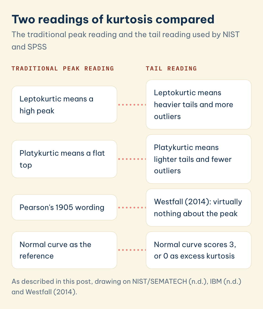
Westfall (2014) records that Pearson introduced the words leptokurtic, mesokurtic and platykurtic for kurtosis above, equal to and below that of the normal curve, and that Pearson himself described them in terms of flat-toppedness. That historical wording is why so many textbooks still link the types to peaks. Kim (2013), writing for clinical researchers, repeats the traditional description, with leptokurtic meaning a high peak and platykurtic a flat-topped curve.
You can keep the three labels and still describe them accurately. A leptokurtic variable, such as income or hospital stay length (often also skewed), usually has a few very large values in the tails. A platykurtic variable, such as scores spread evenly across a scale, has fewer extreme values than a normal curve. Describe what you see in the tails and in your histogram, and use the label as shorthand.
Two readings of kurtosis compared
The traditional peak reading and the tail reading used by NIST and SPSS
Traditional peak reading
Tail reading
Leptokurtic means a high peak
Leptokurtic means heavier tails and more outliers
Platykurtic means a flat top
Platykurtic means lighter tails and fewer outliers
Pearson's 1905 wording
Westfall (2014): virtually nothing about the peak
Normal curve as the reference
Normal curve scores 3, or 0 as excess kurtosis
Save this figure
| Type | Excess kurtosis | Tails compared with normal |
|---|---|---|
| Leptokurtic | Above 0 | Heavier, more outliers |
| Mesokurtic | About 0 | Similar to a normal curve |
| Platykurtic | Below 0 | Lighter, fewer outliers |
◆ Question 4 / 7 · Formula
What is the kurtosis formula?
Direct answer: Kurtosis is the average of the fourth powers of each value's distance from the mean, divided by the standard deviation raised to the fourth power. Subtracting 3 gives excess kurtosis. Because each distance is raised to the fourth power, values far from the mean dominate the result, which is why kurtosis tracks the tails.
NIST/SEMATECH (n.d.) gives the sample formula as the sum of (Yi minus the mean) to the fourth power divided by N, all over s to the fourth power, where s is computed with N rather than N minus 1. Software rarely stops there. Joanes and Gill (1998) compared the different sample estimators used by statistical packages and showed that they give different values in small samples, which is one reason your SPSS figure may not match a hand calculation or another program exactly.
The fourth power is the key to interpretation. A value 3 standard deviations from the mean contributes 81 to the sum, while a value 1 standard deviation away contributes only 1. Westfall (2014) shows that values inside the mean plus or minus one standard deviation contribute at most about 1 to the kurtosis value, so for heavy-tailed data a few extreme cases can move the statistic a long way.
◆ Question 5 / 7 · Skewness vs kurtosis
How are skewness and kurtosis different?
Direct answer: Skewness measures asymmetry, whether one tail is longer than the other. Kurtosis measures tail weight on both sides together, whether the distribution produces more or fewer extreme values than normal. A distribution can be perfectly symmetric, with skewness of 0, and still have very high kurtosis.
IBM (n.d.) defines skewness as a measure of the asymmetry of a distribution, with a positive value showing a long right tail and a negative value a long left tail. Kurtosis answers a different question. The NIST/SEMATECH (n.d.) Cauchy distribution is symmetric in theory, yet its heavy tails pushed the sample kurtosis into the thousands, which shows that tail weight is a separate question from symmetry.
In a dissertation you normally report both in the same descriptive table, with their standard errors. DeCarlo (1997) gives a detailed account of what each statistic captures and how they relate to normality tests, which is useful background if a marker asks you to justify your reading. Our companion guide on quantitative business analysis assignments shows where these statistics usually appear in a coursework report.
◆ Question 6 / 7 · Reading SPSS output
How do you interpret a kurtosis value in SPSS?
Direct answer: Divide the excess kurtosis by its standard error to get a z-score, then compare it with a cut-off that depends on sample size. Kim (2013) suggests 1.96 below 50 cases and 3.29 for 50 to 300 cases. Above 300, judge the histogram and the raw value, with 7 on the original scale as a reference.
IBM (n.d.) explains that the ratio of kurtosis to its standard error can be used as a test of normality, rejecting normality if the ratio is less than minus 2 or greater than plus 2. Kim (2013) refines this by sample size, because standard errors shrink as samples grow, so large samples flag trivial departures while small samples miss real ones. For samples above 300, Kim (2013) follows West et al. in treating an absolute skewness above 2 or an absolute kurtosis (proper) above 7 as substantial departure.
| Sample size | Kim (2013) rule for kurtosis |
|---|---|
| Under 50 | Non-normal if the absolute z-score exceeds 1.96 |
| 50 to 300 | Non-normal if the absolute z-score exceeds 3.29 |
| Over 300 | Use the histogram and the raw value, with absolute kurtosis (proper) above 7 as a reference |
Do not rely on one number alone. Kim (2013) recommends combining visual inspection, skewness and kurtosis, and formal normality tests, then transforming the data or choosing a nonparametric method if the departure is substantial. State in your methods which rule you applied and cite it, so the marker can follow your decision.
◆ Question 7 / 7 · Mentor help
Can a mentor help you report kurtosis correctly?
Many students can produce SPSS output on their own, and reading kurtosis is a skill worth building yourself. A mentor helps with the parts that are hard to judge from inside a project: whether your normality rule fits your sample size, whether a high kurtosis value comes from real outliers or data entry errors, and whether your descriptive table reads clearly to a marker. Through SPSS, R and Python help in your discipline, a MAAS expert works alongside you on your own data, explains each step, and reviews the interpretation you write, with your supervisor's expectations as the reference point.
Frequently asked questions
What is kurtosis in simple terms?
Kurtosis tells you how heavy the tails of a distribution are compared with a normal curve. High kurtosis means more extreme values than normal, and low kurtosis means fewer (NIST/SEMATECH, n.d.).
Does high kurtosis mean a peaked distribution?
Not reliably. Westfall (2014) shows that kurtosis says virtually nothing about the shape of the peak and should be read in terms of tails and outliers.
What does a kurtosis of 3 mean?
It is the value for a normal distribution on the original scale. SPSS subtracts 3 and reports excess kurtosis, so a normal variable shows a value near 0 (IBM, n.d.).
Is negative kurtosis bad?
No. Negative excess kurtosis means lighter tails than a normal curve, a platykurtic shape. It becomes a problem only when the departure is large enough to break the assumptions of your chosen test (Kim, 2013).
What is an acceptable kurtosis value for normality?
It depends on sample size. Kim (2013) uses z-score cut-offs of 1.96 and 3.29 for smaller samples and an absolute kurtosis (proper) of 7 as a reference for samples above 300.
Why does my kurtosis differ between SPSS and Excel?
Programs use different sample estimators and some report excess kurtosis while others do not. Joanes and Gill (1998) show that these estimators differ noticeably in small samples.
References
DeCarlo, L. T. (1997). On the meaning and use of kurtosis. Psychological Methods, 2(3), 292–307. https://doi.org/10.1037/1082-989X.2.3.292
IBM. (n.d.). Descriptives options. IBM SPSS Statistics documentation. https://www.ibm.com/docs/en/spss-statistics/32.0.0?topic=descriptives-options
Joanes, D. N., & Gill, C. A. (1998). Comparing measures of sample skewness and kurtosis. Journal of the Royal Statistical Society: Series D (The Statistician), 47(1), 183–189. https://doi.org/10.1111/1467-9884.00122
Kim, H.-Y. (2013). Statistical notes for clinical researchers: Assessing normal distribution (2) using skewness and kurtosis. Restorative Dentistry & Endodontics, 38(1), 52–54. https://doi.org/10.5395/rde.2013.38.1.52
NIST/SEMATECH. (n.d.). Measures of skewness and kurtosis. e-Handbook of statistical methods. https://www.itl.nist.gov/div898/handbook/eda/section3/eda35b.htm
Westfall, P. H. (2014). Kurtosis as peakedness, 1905–2014. R.I.P. The American Statistician, 68(3), 191–195. https://doi.org/10.1080/00031305.2014.917055
Tools & resources
Not sure how this guide applies to your own case? Talk it through with MAAS in a free 20-minute consultation.
Book a free consultation ▸