
◆ Research Methods
How do you make a frequency distribution table for your data?
Direct answer: List each value or class interval in the first column, count how many observations fall in each, and add that count as a frequency column. Then add relative and cumulative columns. Watts (2025) says classes must not overlap and must cover every observation. Check that the frequencies add up to your sample size n.
◆ Question 1 / 7 · The table
What is a frequency distribution table?
Direct answer: A frequency distribution table is a summary of your data that shows how many observations fall into each of several non-overlapping classes. Watts (2025) uses that definition and treats "frequency table" as a synonym. It often appears early in a results chapter, because it shows the shape of the data before any test.
Watts (2025) defines a frequency distribution as "a summary table of data that shows the number of observations that fall into each of several, non-overlapping classes." The simplest version lists every value once and counts how often it occurs. Watts (2025) works through a small example of daily work hours for 20 students, where the values run from 2 to 7 and the frequencies are 3, 5, 3, 6, 2 and 1. The six frequencies add up to 20, which is the number of students, and that is the first check you should run on any table you build. If the total does not equal your sample size, a value has been missed or counted twice. Once the basic count is right, you can add percentage and cumulative columns, which the sections below explain. For choosing which analysis to run after you have described the data, see our guide on choosing the right statistical test.
◆ Question 2 / 7 · Grouping
When should you group data into class intervals?
Direct answer: Group data into class intervals when the range of scores is wide. Peter (2024) says that when the range is about 20 or less you can list each score, and otherwise you should use intervals. Grouping trades detail for a table short enough to read.
The cut-off Peter (2024) gives is a spread of 20 or fewer between the highest and lowest score: below that, list every value. Peter (2024, section 2.4) illustrates the grouped case with annual salary for 18 people. The table uses 17 intervals of width 10,000, running from 30,000-39,999 up to 190,000-199,999. After counting, Peter (2024) tells readers to add up the frequencies and confirm they equal n, which here is 18. The text also makes a point that many students miss: keep intervals that have a frequency of zero. Peter (2024, p. 2.4.4) puts it directly: "removing those intervals makes the table shorter yet increases the cognitive load", because the reader has to work out that a gap in the scale is a gap in the data. A table that skips from one interval to a distant one hides the very pattern, such as a cluster with a hole beside it, that a frequency table is supposed to reveal. Keep the rows, even when they are empty.
◆ Question 3 / 7 · Classes
How many classes and what class width should you use?
Direct answer: Watts (2025) recommends between five and twenty classes, with fewer classes for smaller data sets. Approximate the class width as (maximum minus minimum) divided by the number of classes, then round up to a convenient number. Every class should have the same width.
Watts (2025) gives a concrete example of the rounding step, where an approximate width of 14.2 is rounded up to 15 because a round number is easier for the reader to use. The same source states that classes must be non-overlapping and exhaustive, meaning each observation belongs to exactly one class, and that all classes share one width. Watts (2025) also stresses that these choices are subjective, so two careful analysts can produce slightly different tables from the same data. A guide that is often mentioned alongside this one is Sturges (1926), which is usually cited as the origin of a rule of thumb for choosing the number of classes from the sample size, commonly stated as k ≈ 1 + 3.322 log10(n). Treat any such rule as a starting point, then adjust until the table is readable and every class has a clear boundary.
◆ Question 4 / 7 · Relative and cumulative
How do you add relative and cumulative frequency?
Direct answer: Relative frequency is each class count divided by n, usually shown as a percentage. Cumulative frequency is a running total of the counts. Peter (2024) states that "The sum of all values in the relative frequency column must be 100% (give or take any rounding error introduced when reporting percentages for each interval)" (p. 2.4.7).
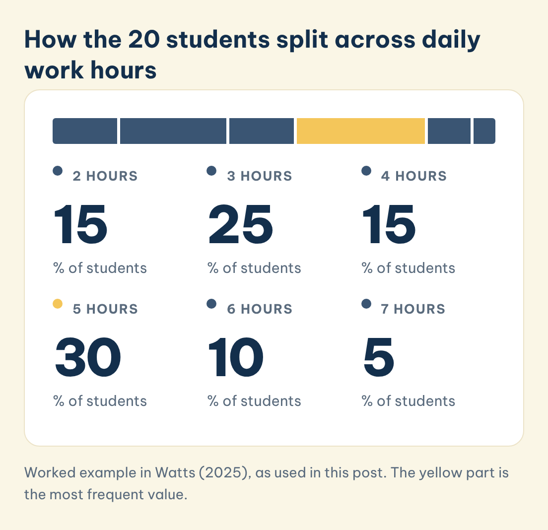
Peter (2024, p. 2.4.7) shows the calculation with the salary data, where one case out of 18 gives (1 ÷ 18) × 100 = 5.56%. Cumulative columns work as running totals. Peter (2024, p. 2.4.6) describes a cumulative column that "counts up from the bottom row to tell how many cases occur at or below each row", because that table lists the highest value at the top. The table in Watts (2025) lists the lowest value first, so its running total goes down the page. Both accumulate from the lowest value, so whichever row order you use, state it in your table note. The worked table below uses the 20-student example from Watts (2025), and each column can be checked against the others.
| Daily work hours | Frequency | Relative frequency | Cumulative frequency | Cumulative relative frequency |
|---|---|---|---|---|
| 2 | 3 | 15% | 3 | 15% |
| 3 | 5 | 25% | 8 | 40% |
| 4 | 3 | 15% | 11 | 55% |
| 5 | 6 | 30% | 17 | 85% |
| 6 | 2 | 10% | 19 | 95% |
| 7 | 1 | 5% | 20 | 100% |
Watts (2025) adds that rounding means the relative frequencies may not sum to exactly 100%, so a total slightly above or below 100% is normally a rounding effect, not an error.
How the 20 students split across daily work hours
Relative frequency in the worked table from Watts (2025). The six shares add up to 100%.
2 hours
15
% of students
3 hours
25
% of students
4 hours
15
% of students
5 hours
30
% of students
6 hours
10
% of students
7 hours
5
% of students
Save this figure
◆ Question 5 / 7 · SPSS
How do you make a frequency table in SPSS (Percent vs Valid Percent)?
Direct answer: In SPSS, choose Analyze > Descriptive Statistics > Frequencies, move your variable into the box and run it. The output gives counts, percentages and cumulative percentages (IBM, n.d.). The step that confuses students is the difference between Percent and Valid Percent when some cases are missing.
IBM (n.d.) documents the Frequencies procedure as producing frequency counts, percentages and cumulative percentages, and notes that these tabulations "provide a useful description for data from any distribution, especially for variables with ordered or unordered categories". The documentation also says the table can be suppressed when a variable has many distinct values, and that rows can be ordered by value or by count. Yeager (2026) uses a class of 435 students to show the difference between the two percentage columns. Of those, 29 are missing class rank and 406 are valid. For freshmen, the count is 147, the Percent is 33.8 (out of all 435) and the Valid Percent is 36.2 (out of the 406 non-missing). Cumulative Percent adds up the Valid Percent values down the rows. If you report the Valid Percent, also say how many cases were missing, so the reader knows the denominator. Yeager (2026) also recommends reading the mode from the frequency table rather than requesting the mode statistic.
◆ Question 6 / 7 · APA 7 reporting
How should you report a frequency table in your dissertation (APA 7)?
Direct answer: Report the count (n) and the percentage (%) in separate columns, and give the total sample size in a table note. The American Psychological Association (n.d.) sample table does this with N = 150 and refers readers to section 7.21 of the Publication Manual for table rules.
The APA sample demographic table in American Psychological Association (n.d.), which points to section 7.21 of the Publication Manual, shows the pattern clearly: one row per category, a column for n, a column for percentage, and a note that states the total. Following that layout means a reader can check your percentages without asking where the denominator came from. If any cases are missing, say so in the note, because the denominator then changes, as the Percent and Valid Percent example above shows. Keep the table close to the sentence that discusses it, and describe the main pattern in words rather than repeating every number. Your department may add its own formatting conventions, so check the handbook before you finalise the layout. For wider guidance on presenting and interpreting numbers across a whole thesis, see our guide to thesis statistics help.
◆ Question 7 / 7 · Getting help
How can MAAS help you build and read your frequency tables?
Direct answer: MAAS works as a mentor and advisor. An expert in the SPSS, R and Python data analysis service can talk through your variables, show you how to read the SPSS output, and review your table layout, so you understand every number you report. The first 20-minute discovery call is free.
Many students arrive with a data file and a deadline but no clear picture of which output belongs in the results chapter. A mentor can look at your variable types, explain why one variable needs class intervals and another does not, and help you spot where Percent and Valid Percent could be confused. The mentor guides and reviews. You run the procedures, make the choices and write the chapter in your own words. That split keeps the work yours while still giving you someone to check your reasoning against. If you are unsure what to do after the descriptive stage, the guide on choosing the right statistical test is a sensible next read.
Frequently asked questions
What is the difference between a frequency table and a relative frequency table?
A frequency table gives counts, and a relative frequency table gives each count as a share of n, usually in percent. Peter (2024) shows (1 ÷ 18) × 100 = 5.56% as an example.
Do the relative frequencies have to add up to 100%?
Yes, apart from rounding. Both Peter (2024) and Watts (2025) note that rounding each percentage can leave the column total a little above or below 100%.
How many classes should my table have?
Watts (2025) suggests between five and twenty, with fewer for smaller data sets. Peter (2024) says that if the range of scores is about 20 or less, you can list each score instead of grouping.
Should I delete class intervals with zero cases?
No. Peter (2024) says removing empty rows makes the table shorter yet increases the cognitive load for the reader, so keep them.
What is the difference between Percent and Valid Percent in SPSS?
Percent is out of all observations including missing cases, and Valid Percent is out of the non-missing cases. Yeager (2026) shows 33.8 versus 36.2 for 147 freshmen when 29 of 435 cases are missing.
What should the table note say in APA 7?
Give the total sample size, as the sample table in American Psychological Association (n.d.) does with N = 150, and mention any missing cases that change the denominator.
Related guides
References
American Psychological Association. (n.d.). Sample tables. APA Style. https://apastyle.apa.org/style-grammar-guidelines/tables-figures/sample-tables
IBM. (n.d.). Frequencies. IBM SPSS Statistics 32.0.0 documentation. https://www.ibm.com/docs/en/spss-statistics/32.0.0?topic=features-frequencies
Peter, C. R. (2024). Statistics: Open for everyone. LibreTexts. https://batch.libretexts.org/print/Letter/Finished/stats-49315/Full.pdf
Sturges, H. A. (1926). The choice of a class interval. Journal of the American Statistical Association, 21(153), 65-66. https://doi.org/10.1080/01621459.1926.10502161
Watts, V. (2025). Introduction to statistics (2nd ed.). eCampusOntario Pressbooks. https://ecampusontario.pressbooks.pub/introstats2ed/chapter/2-1-frequency-distributions/
Yeager, K. (2026). SPSS tutorials: Frequency tables. Kent State University Libraries. https://libguides.library.kent.edu/SPSS/FrequenciesCategorical
Not sure how this guide applies to your own case? Talk it through with MAAS in a free 20-minute consultation.
Book a free consultation ▸