
◆ Research Methods
What are degrees of freedom in statistics, in plain English?
Degrees of freedom are the number of values in your data that are free to vary once your calculation has fixed some quantity, such as the mean. Most software prints a "df" figure beside every test, and most students copy it without knowing where it came from. This guide shows where it comes from, test by test.
◆ Question 1 / 9 · What it is
What is a degree of freedom in statistics?
Direct answer: A degree of freedom is one value in your data that can still vary freely after your analysis has imposed its constraints. Frost (2017) defines the term as the number of independent values that can vary without breaking any constraints. The usual count is the number of observations minus the number of quantities you estimated from them.
Walker (1940) opens a classic article by saying that this is "A concept of central importance to modern statistical theory which few textbooks have attempted to clarify" (Walker, 1940, p. 253). He adds that for readers without the geometry behind it, the idea "often seems almost mystical, with no practical meaning" (Walker, 1940, p. 253). The practical meaning is simpler than that opening suggests. Colorado State University (n.d.) puts it as a subtraction: "the number of quantities that went into the calculation − the number of constraints they must satisfy".
Gauss, as Walker (1940) records, stated that the number of observations is to be decreased by the number of unknowns estimated from the data, which is the same subtraction. A worked example makes this concrete. Suppose you have 3 numbers and you are told their mean is 10, so they must add up to 30. You can choose the first number freely, say 8, and the second freely, say 13. The third is now forced: 30 − 8 − 13 = 9. Only 2 of the 3 values could vary, so the data carry 2 degrees of freedom, which is n − 1 with n = 3. The mean was the one constraint, and each constraint costs one degree of freedom. That is why the same rule shows up again and again below: count what you have, then subtract what you had to estimate.
◆ Question 2 / 9 · In a test
What is meant by degree of freedom when you run a test?
Direct answer: In a test, degrees of freedom tell the software which version of the reference distribution to use. The t distribution has only one parameter, its degrees of freedom, which is based on but not equal to the sample size (Frost, 2022). A different df gives a different critical value, so it changes your verdict.
Small samples give a wider, heavier-tailed t curve, because an estimate built from few independent values is less certain. Frost (2022) notes that at around 30 degrees of freedom the t distribution closely approximates the standard normal distribution. That is why textbooks often treat 30 as a rough turning point, although it is a convention rather than a rule.
Regression shows the same logic from the other side. Tupper (2023) writes that the model "uses up" the degrees of freedom in your dataset when it finds the parameter estimates. Frost (2017) gives the numbers: with n = 29 and two predictors, the total df is 28 and the error df is n − P − 1 = 26, and as you add terms to the model the error degrees of freedom decrease. Every predictor you add is one more thing estimated from the same data, so fewer values are left to judge how well the model fits.
◆ Question 3 / 9 · Formulas
What is the degree of freedom formula for each test?
Direct answer: The rule is df = N − P, the number of observations minus the number of parameters estimated (Frost, 2017). In practice you memorise a few patterns: n − 1 for one sample and paired data, N − 2 for two groups and Pearson r, k − 1 and N − k for one-way ANOVA, and (r − 1)(c − 1) for chi-square independence.
The table collects the formulas that most dissertations need. It follows Colorado State University (n.d.), Frost (2017) and Tupper (2023), with the Welch row from Welch (1947).
| Test | Degrees of freedom | Where the subtraction comes from |
|---|---|---|
| One-sample t | n − 1 | One mean estimated |
| Paired t | pairs − 1 | The differences form one sample |
| Independent t (equal variances) | n1 + n2 − 2 | Two group means estimated |
| Welch t (unequal variances) | Approximate, often fractional | Welch's adjustment (1947) |
| Pearson r | n − 2 | Two parameters (intercept and slope of the fitted line) |
| Simple regression (t for the slope) | n − 2 | Intercept and slope estimated |
| Multiple regression (t per predictor) | n − k − 1 | Intercept plus k slopes estimated |
| One-way ANOVA, between groups | k − 1 | k group means around one grand mean |
| One-way ANOVA, within groups | N − k | k group means estimated |
| Chi-square goodness of fit | k − 1 | Total count fixed |
| Chi-square independence | (r − 1)(c − 1) | Row and column totals fixed |
Introductory courses usually lean on 6 of these 11 rows: one-sample t, paired t, independent t, Pearson r, one-way ANOVA and chi-square independence, while the regression rows appear once you reach SPSS or Python output. Notice that the table never asks for anything beyond counting. If your design is not on this list, ask which quantities your software estimated before it reached the test statistic, and subtract them from the number of independent values. Our guide to choosing the right statistical test helps you pick the row before you worry about its df.
◆ Question 4 / 9 · t test
How do you calculate degrees of freedom for a t test?
Direct answer: For a one-sample t test use n − 1. For a paired t test use the number of pairs minus 1. For an independent-samples t test with equal variances use n1 + n2 − 2. If Levene's test says the variances differ, use the Welch row, whose df is approximate and often fractional.
Frost (2017) writes the general rule as DF = N − P, and Colorado State University (n.d.) lists N − 2 for the two-sample t test with equal variance. Take two groups of 15 students each. The pooled independent-samples test has 15 + 15 − 2 = 28 degrees of freedom, because two group means were estimated. You would write the result as t(28) = 2.10. A paired design with 15 students measured twice has only 15 − 1 = 14 degrees of freedom, because the 15 differences form a single sample.
Patel (n.d.) explains that Levene's test checks the homogeneity of variance, and that when this assumption is not met you should not use the pooled estimate. In SPSS output, that means reading the Welch row instead. Welch (1947) is the origin of the approximate df used there, so a value such as 24.37 is normal output, not an error. Report it to the decimals your software prints, since changing it to a whole 28 would misstate which test you ran.
◆ Question 5 / 9 · n − 1 or n − 2
When should you use n − 1 or n − 2 degrees of freedom?
Direct answer: Use n − 1 when you estimate one parameter, the mean, from a single set of values. Use N − 2 when you estimate two, such as two group means in an independent t test, or the two parameters behind a Pearson correlation. The choice follows from how many quantities your calculation had to estimate.
When n − 1 and when n − 2
How many quantities your calculation had to estimate
n − 1 degrees of freedom
N − 2 degrees of freedom
One parameter estimated: the mean
Two parameters estimated
One-sample t test
Independent t test with two group means
Paired t test: pairs − 1
Pearson r: n − 2
Three numbers with mean 10 leave 2 free
Simple regression: intercept and slope
Save this figure
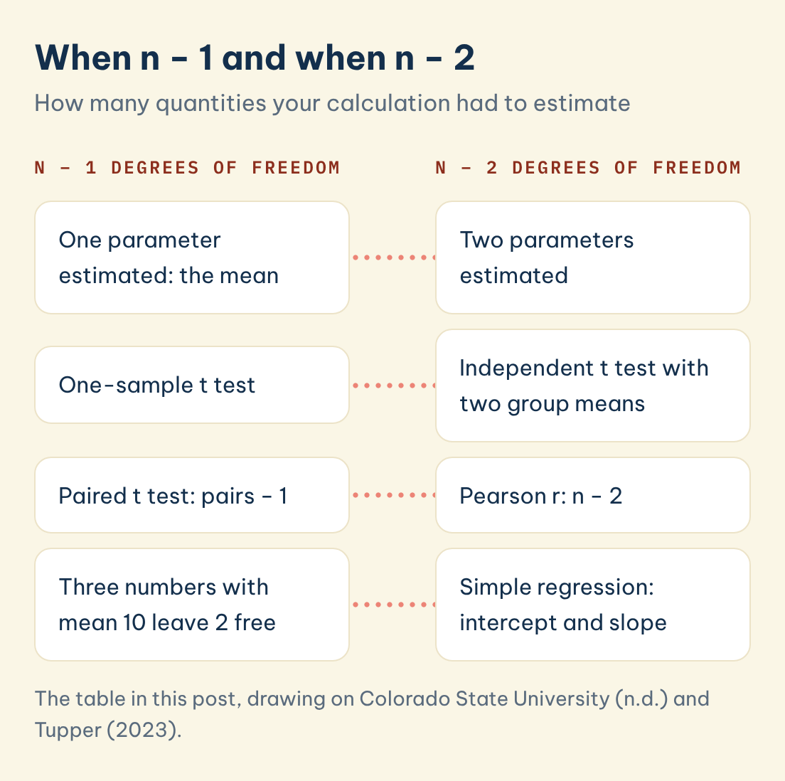
The rule in everyday terms is simple. With one sample, the mean is the only thing estimated, so you lose one degree. With two groups, each group mean is estimated, so you lose two. A correlation is equivalent to a simple regression, so Pearson r also uses n − 2. Simple linear regression reaches the same n − 2 for a different reason, since it estimates an intercept and a slope (Tupper, 2023). Multiple regression extends it to n − k − 1 where k is the number of predictors.
The confusion usually arises because students memorise the numbers instead of the reason. If you remember the count-and-subtract rule from the first section, you can rebuild every row of the table on the spot, and you will also notice when software reports something unusual. A one-way ANOVA is a good test of the habit: between groups you have k − 1, and within groups N − k, which together add up to N − 1 (Colorado State University, n.d.). The total always matches the one-sample count, because the grand mean is the single constraint on all the data.
◆ Question 6 / 9 · Chi-square
What are degrees of freedom in chi-square?
Direct answer: For a chi-square test of independence, df = (r − 1)(c − 1), where r and c are the numbers of rows and columns in the table (Colorado State University, n.d.). For a goodness-of-fit test it is k − 1, where k is the number of categories. The totals are fixed, so the last cell is forced.
Colorado State University (n.d.) illustrates this with a 2 × 2 table: with the margins fixed, once you fill in any one cell the other three are forced. That is why the table has (2 − 1)(2 − 1) = 1 degree of freedom, even though it holds four cells. A 3 × 4 table has (3 − 1)(4 − 1) = 6.
APA style writes the chi-square symbol followed by the degrees of freedom and the sample size in brackets, for example χ²(1, N = 120). The df sits first, then the sample size. The same convention is covered in our guide to reporting effect sizes and confidence intervals.
◆ Question 7 / 9 · The t table
How do degrees of freedom change the t table?
Direct answer: As degrees of freedom increase, the two-tailed critical t value at the .05 level falls toward 1.960. It is 2.571 at df = 5, 2.228 at df = 10, 2.086 at df = 20, 2.042 at df = 30, and 1.960 with infinite df. A larger sample therefore needs a smaller t to reach significance.
| Degrees of freedom | Two-tailed critical t at .05 |
|---|---|
| 5 | 2.571 |
| 10 | 2.228 |
| 20 | 2.086 |
| 30 | 2.042 |
| Infinite | 1.960 |
Read the table from the top: at df = 5 the bar is 2.571, at df = 10 it drops to 2.228, and with infinite df it settles at 1.960, which is the familiar normal-curve value. Frost (2017) gives the same reading for the middle of the table: for a two-tailed t test with 20 degrees of freedom and an alpha of 0.05, the critical values are −2.086 and +2.086. A result of t = 2.10 clears that bar at df = 20 and at df = 30, but it would not clear the bar at df = 10. The statistic is identical in each case. Only the degrees of freedom changed, and with them the verdict.
Quoting df beside every statistic matters: a reader cannot judge a t of 2.10 without knowing how many independent values stood behind it. The table also explains a common feeling, that small studies need a bigger effect to count as significant. They do, because a small sample leaves little information to separate a real difference from noise.
◆ Question 8 / 9 · APA 7
How do you report degrees of freedom in APA 7?
Direct answer: Put the degrees of freedom in brackets straight after the statistic symbol, as in t(28) = 2.10. An F test takes two df, such as F(3, 906), and chi-square adds the sample size, as in χ²(1, N = 120) (American Psychological Association, n.d.). Report the df your software printed, including fractional Welch values.
A full sentence for the two-group example reads: the treatment group scored higher than the control group, t(28) = 2.10. Because the exact p value should come from your software, copy it from the output rather than reading it off the t table. The table only brackets the answer. If you want a refresher on formatting the rest of the sentence, the effect size guide linked above shows how to add the interval and the magnitude.
Colorado State University (n.d.) gives F(3, 906) as its example of an F test: 3 degrees of freedom for the groups and 906 for the error term. Students quote N instead of df, forget that ANOVA has two df, or round a Welch df to a whole number. Check each statistic in your results chapter against the table above and ask whether the df makes sense for the design. If it does not match, the usual culprit is a miscounted sample or the wrong test row.
◆ Question 9 / 9 · Mentor help
Can a mentor help you with degrees of freedom and test output?
If your supervisor has flagged your results chapter, Data & Coding Projects lets you work through your own output with a MAAS expert alongside you, covering which test fits your design, what each number in your SPSS or Python output means, and how to report it. You stay the author throughout, and your institution decides what the work earns, so there is no promise about grades. Send your dataset description and the output you do not understand, and the mentor will walk you through the logic until you could explain it to your marker.
Frequently asked questions
What is a degree of freedom in statistics?
It is the number of independent values that can vary in an analysis without breaking any constraints (Frost, 2017). The usual count is observations minus the quantities you estimated.
Is 0.01 or 0.05 more significant?
A p value of .01 is smaller than .05, so it is stronger evidence against the null hypothesis. Both only tell you about chance, not size, so pair them with an effect size, as in our guide to reporting effect sizes and confidence intervals.
When do I use n − 1 or n − 2 degrees of freedom?
Use n − 1 for one sample or paired data, and N − 2 for two independent groups or a Pearson correlation. The general rule is df = N − P (Frost, 2017).
What is the degree of freedom formula for chi-square?
Use (r − 1)(c − 1) for a test of independence (Colorado State University, n.d.), and k − 1 for goodness of fit, because the total count is fixed.
Why does my Welch t test show a decimal df?
Welch (1947) gave an approximate df for unequal variances, so a fractional value is normal output. Report it as printed.
Can degrees of freedom be zero or negative?
With n − 1 you reach zero when n = 1, and then there is nothing left to estimate variability from. A negative value means you estimated more parameters than you have observations, so the model cannot be fitted.
References
American Psychological Association. (n.d.). Numbers and statistics. APA Style. https://apastyle.apa.org/style-grammar-guidelines/numbers/statistics
Colorado State University. (n.d.). Conducting common hypothesis tests. PSY 652: Methods of Research in Psychology I. https://psy652.colostate.edu/modules/m09-conducting-NHST.html
Frost, J. (2017). Degrees of freedom in statistics. Statistics By Jim. https://statisticsbyjim.com/hypothesis-testing/degrees-freedom-statistics/
Frost, J. (2022). T distribution: Definition & uses. Statistics By Jim. https://statisticsbyjim.com/probability/t-distribution/
Patel, C. (n.d.). Tutor's quick guide to statistics. statstutor, Loughborough University. https://statstutor.lboro.ac.uk/resources/uploaded/tutorsquickguidetostatistics.pdf
Tupper, L. (2023). Degrees of freedom. In Stat 340 notes: Fall 2023. https://bookdown.org/ltupper/340f23_notes/degrees-of-freedom.html
Walker, H. M. (1940). Degrees of freedom. Journal of Educational Psychology, 31(4), 253–269. https://doi.org/10.1037/h0054588
Welch, B. L. (1947). The generalization of "Student's" problem when several different population variances are involved. Biometrika, 34(1–2), 28–35. https://doi.org/10.1093/biomet/34.1-2.28
Not sure how this guide applies to your own case? Talk it through with MAAS in a free 20-minute consultation.
Book a free consultation ▸